Simultaneous Multi-plane Imaging of Neural Circuits

Abstract

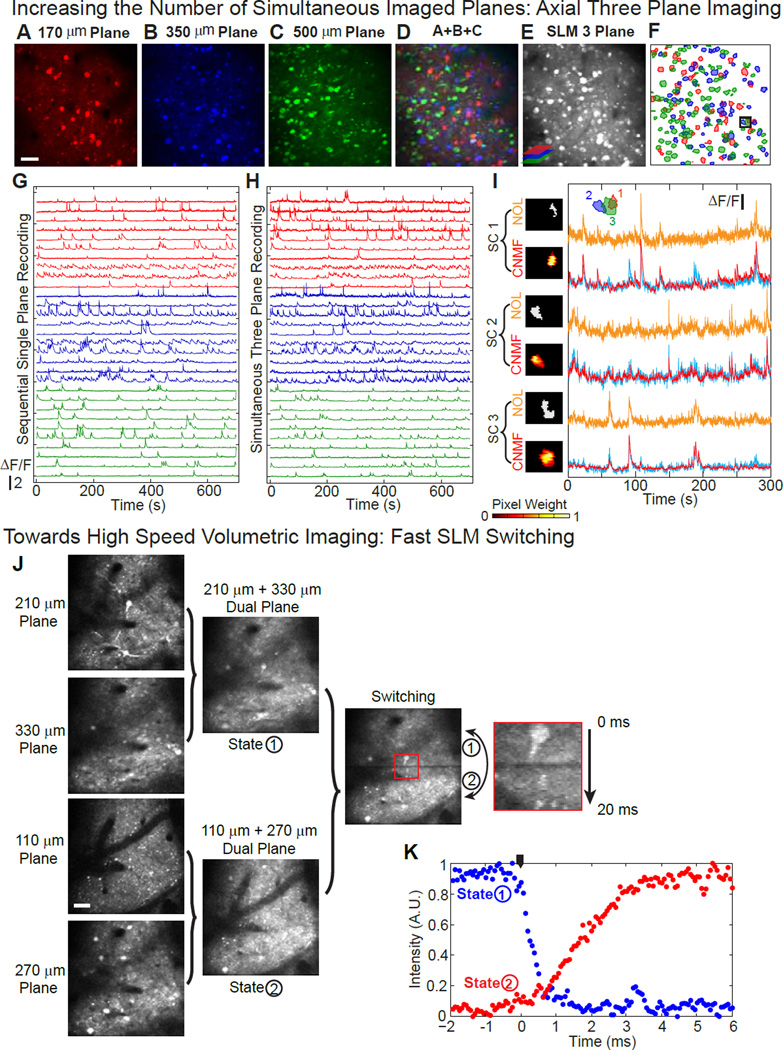
Recording the activity of large populations of neurons is an important step toward understanding the emergent function of neural circuits. Here we present a simple holographic method to simultaneously perform two-photon calcium imaging of neuronal populations across multiple areas and layers of mouse cortex in vivo. We use prior knowledge of neuronal locations, activity sparsity, and a constrained nonnegative matrix factorization algorithm to extract signals from neurons imaged simultaneously and located in different focal planes or fields of view. Our laser multiplexing approach is simple and fast, and could be used as a general method to image the activity of neural circuits in three dimensions across multiple areas in the brain.

Figure 1. SLM Two-photon Microscope and Multiplane Structural Imaging

(A) SLM two-photon microscope. The laser beam from the Ti:Sapphire laser is expanded to illuminate the SLM. The spatially-modulated reflected beam from the SLM passes through a telescope, followed by an XY galvanometric mirror, and directed into a two-photon microscope. This setup is essentially composed of a conventional two-photon microscope, and an SLM beam shaping component (red dashed box). (B) Illustration of axial dual plane imaging, where two planes at different depths can be simultaneously imaged. (C) Illustration of lateral dual plane imaging, where two fields of view at the same depth can be simultaneously imaged. (D) Two-photon structural imaging of a shrimp at different depths through the sample, obtained by mechanically moving the objective with a micrometer. Each imaging depth is pseudo-colored. The last image is constructed by overlaying all other images together. Scale bar, 100 µm. (E) Software based SLM focusing of the same shrimp as (D). The SLM is used to modify the wavefront of the light to control the focal depth, while the position of the objective is fixed. The nominal focus of the objective is fixed at the 100 µm plane. This set of images looks similar to that in (D). Scale bar, 100 µm. (F) Arithmetic sum of all the images at the seven planes shown in (D). (G) Arithmetic sum of all the images at the seven planes shown in (E). (H) Seven-axial-plane imaging of the same shrimp as (D)–(G), using the SLM to create 7 beamlets that simultaneously target all seven planes. (I) Same as (H), but using the SLM to increase the illumination intensity only for the 50 µm plane. Features on that plane are highlighted compared to panel (H). Scale bar, 100 µm.

Figure 2. Lateral Dual Plane in-vivo Functional Imaging of Mouse V1

(A) Schematic of the in-vivo experiment, imaging V1 in the mouse. In this experiment, two fields of view (FOV), laterally displaced by 300 µm, are simultaneously imaged. (B) /(C) Top panel, temporal standard deviation image of the sequential single plane recording (10 fps) of FOV 1 (B), and FOV 2 (C), of mouse V1 at a depth of 280 µm from the pial surface. Bottom panel, spatial component contours overlaid on the top panel. The boxes in dashed line show the overlapped region, shared in both FOVs. Scale bar, 50 µm. (D) Arithmetic sum of (B) and (C). (E) Top panel, temporal standard deviation image of the simultaneous dual plane recording (10 fps) of the two FOVs. Bottom panel, overlaid spatial component contours from the two FOVs. (F) Representative extracted ΔF/F traces, using the CNMF algorithm, of the selected spatial components from the two field of views (red, FOV 1; green, FOV 2), from the sequential single plane recording. (G) Extracted ΔF/F traces, using the CNMF algorithm, of the same spatial components shown in (F), from the simultaneous dual plane recording. The areas highlighted in blue in the dual plane ΔF/F traces are two spatial components taken from the overlapped area of the two FOVs. Their spatial contours are shown with the black box in the bottom panel in (E). (H) Zoomed view of the ΔF/F traces in the shaded area in (G), showing the extremely high correlation between the independently extracted dynamics from the twinned spatial components.

Figure 3. Axial Dual Plane in-vivo Functional Imaging of Mouse V1 at Layer 2/3 and 5

(A) Schematic of the in-vivo experiment, imaging V1 in the mouse. In this experiment, two different planes, axially separated by 330 µm, are simultaneously imaged. (B) / (C) Top panel, temporal standard deviation images of the sequential single plane recording (10 fps) of mouse V1 at depth of 170 µm (layer 2/3) and depth of 500 µm (layer 5) from the pial surface. The images are false-colored. Bottom panel, spatial component contours overlaid on the top panel. Scale bar, 50 µm. (D) Arithmetic sum of (B) and (C). (E) Top panel, temporal standard deviation image of the simultaneous dual plane (10 fps) recording of the two planes shown in (B) and (C). Bottom panel, overlaid spatial component contours from the two planes. (F) Representative extracted ΔF/F traces, using the CNMF algorithm, of 20 spatial components out of 345 from the two planes (red, layer 2/3; green, layer 5), from the sequential single plane recording. (G) Extracted ΔF/F traces, using the CNMF algorithm, of the same spatial components shown in (F), from the simultaneous dual plane recording. (H) / (I) Zoomed in view of the extracted ΔF/F traces in the shaded area in (F) and (G) respectively. (J) Further enlargement of the small events in the ΔF/F traces shown in the blue shaded areas in (H) and (I).

Figure 4. Source Separation

Source separation of the fluorescent signal from spatially overlapped spatial components (SCs) in the dual plane images shown in Fig 3. (A) and (B) show two different examples with increasing complexity. In each example, the contours of the overlapped spatial components are plotted in red (from layer 2/3) and green (from layer 5) with their source ID. A pixel maximum projection of the recorded movie are shown to illustrate the spatial overlap of these SCs. Raw image frames from the recorded movie show the neuronal activity of these individual spatial components. For the temporal traces, the first trace (in gray) shows that extracted from all the pixels of the overlapped SCs. The following traces show the demixed signal of the individual SCs. Three different methods are used to extract the signal from individual SCs: non-overlapped pixel (NOL), with the extracted signal shown in orange, independent component analysis (ICA) in green, and constrained non-negative matrix factorization (CNMF) in red. The corresponding SC contours result from these methods are shown next to their ΔF/F traces, and the color code of the pixel weighting is shown immediately below (B). Using the SC contour from CNMF, but with uniform pixel weighting and without temporal demixing, the extracted ΔF/F trace is plotted in cyan, superimposed onto the traces extracted from CNMF. In (B), ICA fails to find the spatial component 2. The traces are plotted independently scaled for display convenience. The scaling applied is as follows: the scale bar of ΔF/F is 1.27 for SC 1 and 1.46 for SC 2 in (A); 1.24 for SC 1, 0.48 for SC 2, 0.36 for SC 3, 0.24 for SC 4, 0.78 for SC 5, 0.85 for SC 6, and 0.79 for SC 7 in (B).

Figure 5. Comparison between CNMF and NOL

(A) Correlation coefficient between the ΔF/F extracted from CNMF and NOL for a total of 250 spatial components (SCs) in the dual plane imaging shown in Fig. 3. The blue dashed line indicates the median (0.947) of the correlation coefficients. The SC IDs are sorted by the SNR of the signals extracted by NOL. (B) Signal to noise ratio (SNR) comparison between the ΔF/F extracted from CNMF (with residue) and the ΔF/F extracted from NOL for the 250 SCs. The overall SNR of CNMF (with residue) is 13% higher than that from NOL. (C) An example where three sources that are spatially overlapped in the dual plane imaging is studied. The contours of the overlapped SCs are plotted in red (from layer 2/3) and green (from layer 5) with their spatial component ID. The CNMF and NOL extracted ΔF/F signals are plotted in red and orange respectively. The signal that CNMF extracted, with residual noise is plotted in blue. Using the SC contour in the CNMF but with uniform pixel weighting and without temporal demixing, the extracted ΔF/F trace is plotted in gray, and labelled as “Raw”. The corresponding correlation and SNR values for these two SC are labelled in (A) and (B). The traces are plotted independently scaled for display convenience. The scaling applied is as follows: the scale bar of ΔF/F is 0.29 for SC 1, 0.14 for SC 2, and 0.51 for SC 3. (D) / (E) Histogram of the ΔF/F noise for (D) SC 1 and (E) SC 2. The orange color shows that for the NOL extracted signal, whereas blue shows that for CNMF with residue. The histograms are fitted with a Gaussian function, shown as a solid-line curve.

Figure 6. Orientation and Direction Selectivity Analysis with Simultaneous Dual Plane Imaging

(A) Normalized ΔF/F traces for selected spatial components (SCs) with strong response to drifting grating visual stimulation, recorded with simultaneous dual plane imaging. The red and green color traces are from SCs at depths of 200 µm and 450 µm from the pial surface of mouse V1. The color bar in the bottom of each trace indicates the visual stimulation orientation of the drifting grating, with the legend shown on top of (B), i.e. red: 0°/180°, yellow: 45°/225°, green: 90°/270°, purple: 135°/315°. (B) Left panel, response of the SCs to the drifting grating in visual stimulation. The SCs are on the 200 µm plane. The SCs are separated into four groups, corresponding to a preferred orientation angle of 0°/180°, 45°/225°, 90°/270°, and 135°/315°. The black curves are the average response of the group. Right panel, comparison of the SCs’ preferred orientation angle to the drifting gratings, between signals extracted from the single plane recording (blue dots) and the dual plane recording (orange dots). (C) Same as (B), for spatial components located at 450 µm depth from pial surface. (D) Left, overlaid temporal standard deviation image (with false color) of the sequential single plane recording from the 200 µm plane (red) and from the 450 µm plane (green). Right, extracted SC contours from the two planes. Scale bar, 50 µm. (E) Examples of the evoked responses of the SCs with spatial lateral overlaps from the two planes. The blue color shows that extracted from single plane recording, and the orange shows that extracted from dual plane recording. The arrow inside each SC indicates its preferred direction. The locations of these SCs are indicated in the small black boxes in the SC contours in (D).

Figure 7. Axial Three Plane in-vivo Functional Imaging of Mouse V1, and Fast SLM Switching between Different Holograms

(A) – (C) Temporal standard deviation image of the sequential single plane recording (10 fps) of mouse V1 at depths of 170 µm, 350 µm and 500 µm from the pial surface. The images are false-colored. Scale bar, 50 µm. (D) Arithmetic sum of (A) – (C). (E) Temporal standard deviation image of the simultaneous three-plane recording (10 fps) of the same planes shown in (A) – (C). (F) Overlaid spatial component (SC) contours from the three planes. (G) Representative extracted ΔF/F traces of the selected SCs from the three planes (red, 170 µm plane, 10 SCs out of 58; blue, 350 µm plane, 10 SCs out of 65; green, 500 µm depth, 10 SCs out of 95), from the sequential single plane recording. (H) Extracted ΔF/F traces of the same SCs shown in (G), from the simultaneous three-plane recording. (I) An example of source separation of the fluorescent signal from spatially overlapped components in the three plane imaging. The locations of these SCs are shown in the small black box in (F). The contours of the overlapped SCs are plotted in color with their SC ID. For each SC, the signal is extracted using NOL shown in orange, and CNMF in red. The corresponding SC contours result from these methods are shown next to their ΔF/F traces. A raw trace, generated from the CNMF SC, but with uniform pixel weighting, and without temporal demixing, is plotted in cyan, superimposed onto the traces extracted with CNMF. Fluorescent traces are independently scaled for display convenience. The scale bar of ΔF/F is 0.268, 0.376, and 0.351 for SC 1–3 respectively. (J) SLM switching between two sets of dual plane imaging on mouse V1. State 1 is the dual plane for depth of 210 µm and 330 µm from pial surface, and state 2 is the dual plane for depth of 110 µm and 270 µm from pial surface. Imaging frame rate is 10 fps. The SLM switching happens at the middle and at the end of each frame. The zoom-in-view of the switching region shows that the switching time between the two state is less than 3 ms. Scale bar, 50 µm. (K) SLM switching time between two different states, measured from the change in fluorescent signal emitted from spatially localized planes of Rhodamine 6G. The switching time between different states is less than 3 ms. The black indicator marks when the switching starts.

References

1. Ahrens MB, Orger MB, Robson DN, Li JM, Keller PJ. Whole-brain functional imaging at cellular resolution using light-sheet microscopy. Nature Methods. 2013;10:413–420. - PubMed
1. Alivisatos AP, Andrews AM, Boyden ES, Chun M, Church GM, Deisseroth K, Donoghue JP, Fraser SE, Lippincott-Schwartz J, Looger LL, et al. Nanotools for Neuroscience and Brain Activity Mapping. Acs Nano. 2013a;7:1850–1866. - PMC - PubMed
1. Alivisatos AP, Chun M, Church GM, Deisseroth K, Donoghue JP, Greenspan RJ, McEuen PL, Roukes ML, Sejnowski TJ, Weiss PS, et al. The Brain Activity Map. Science. 2013b;339:1284–1285. - PMC - PubMed
1. Alivisatos AP, Chun M, Church GM, Greenspan RJ, Roukes ML, Yuste R. The Brain Activity Map Project and the Challenge of Functional Connectomics. Neuron. 2012;74:970–974. - PMC - PubMed
1. Andresen V, Egner A, Hell SW. Time-multiplexed multifocal multiphoton microscope. Optics Letters. 2001;26:75–77. - PubMed
Publication types