A Tutorial Review of Functional Connectivity Analysis Methods and Their Interpretational Pitfalls

Abstract

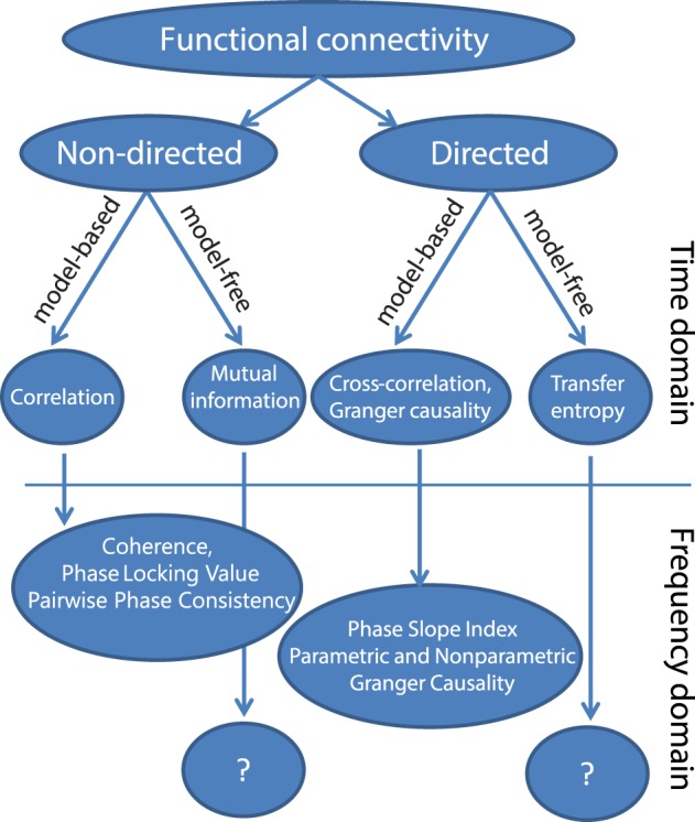
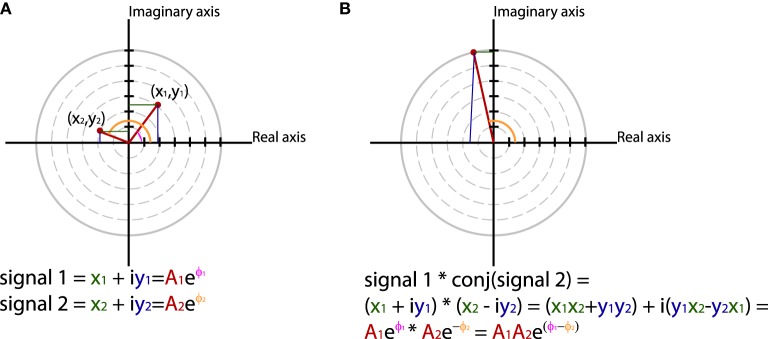
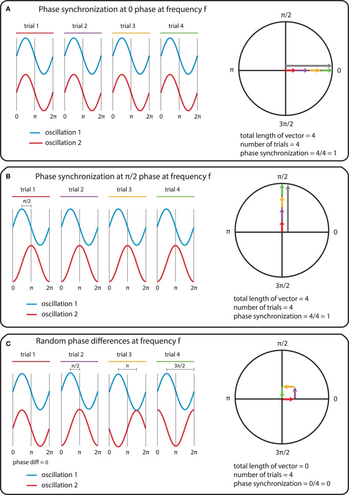
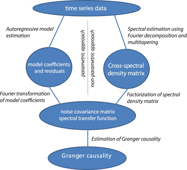
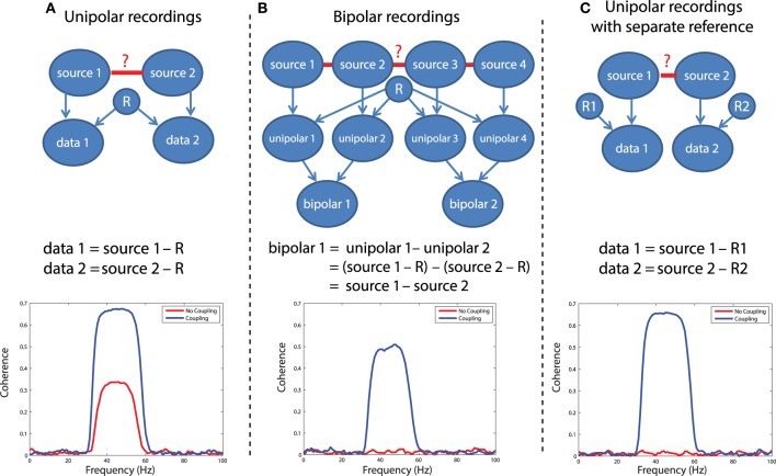
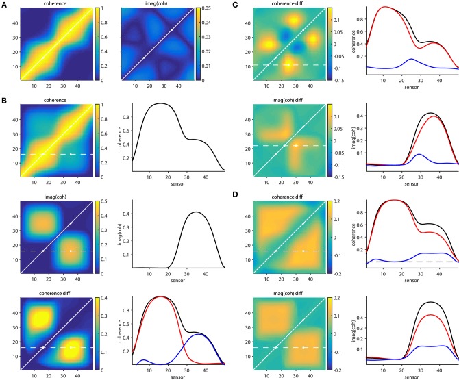
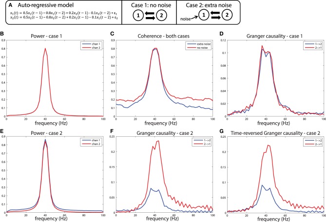
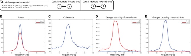
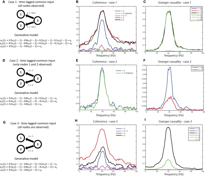
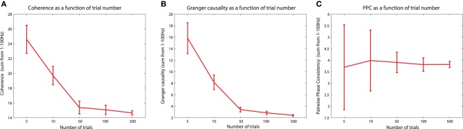
Oscillatory neuronal activity may provide a mechanism for dynamic network coordination. Rhythmic neuronal interactions can be quantified using multiple metrics, each with their own advantages and disadvantages. This tutorial will review and summarize current analysis methods used in the field of invasive and non-invasive electrophysiology to study the dynamic connections between neuronal populations. First, we review metrics for functional connectivity, including coherence, phase synchronization, phase-slope index, and Granger causality, with the specific aim to provide an intuition for how these metrics work, as well as their quantitative definition. Next, we highlight a number of interpretational caveats and common pitfalls that can arise when performing functional connectivity analysis, including the common reference problem, the signal to noise ratio problem, the volume conduction problem, the common input problem, and the sample size bias problem. These pitfalls will be illustrated by presenting a set of MATLAB-scripts, which can be executed by the reader to simulate each of these potential problems. We discuss how these issues can be addressed using current methods.

Keywords: coherence analysis; electrophysiology; functional connectivity (FC); granger causality; oscillations; phase synchronization.

Figure 1

A taxonomy of popular methods for quantifying functional connectivity.

Figure 2

Using polar coordinates and complex numbers to represent signals in the frequency domain. (A) The phase and amplitude of two signals. (B) The cross-spectrum between signal 1 and 2, which corresponds to multiplying the amplitudes of the two signals and subtracting their phases.

Figure 3

The mechanics of the computation of phase synchrony. (A) An instance of perfect phase alignment at 0 radians. (B) An instance of perfect synchronization at a difference of π/2 radians. (C) Absence of phase synchronization due to inconsistent phase differences.

Figure 4

Data processing pipeline for the computation of Granger causality, using the parametric or non-parametric approach.

Figure 5

Illustration of different referencing schemes and how each effects the calculation of coherence with and without true neuronal coupling. (A) The case of unipolar recordings, which introduce spurious coherence values in the absence of coherence. (B) The bipolar derivation technique, which largely resolves the common reference problem. (C) The separate reference scheme, which also is not sensitive to common reference problems.

Figure 6

Effects of field spread on the estimation of connectivity. (A) In absence of connectivity, field spread leads to spurious coherence (left panel), while the imaginary part of coherency mitigates this effect (right panel). (B) In the presence of time-lagged interactions, “seed blur” caused by field spread leads to only a “shoulder” in the coherence, and not to a distant peak (top right panel). The imaginary part of coherency correctly identifies a distant peak (middle right panel). Bottom panels: the distant coherence peak is revealed when taking the difference (blue line) between the connected (black line) and unconnected (red line) situations. (C) Spurious differential effects show up both in the coherence (top panels) and in the imaginary part of coherency (bottom panels) when the SNR changes from one condition to another. (D) Spurious differential effects show up both in the coherence (top panels) and in the imaginary part of coherency (bottom panels) when the amplitude of one of the active sources changes from one condition to another.

Figure 7

A simulation of the signal to noise ratio problem. (A) Two nodes interact bidirectionally with equal connectivity strengths in the two directions, and the data is observed without (case 1) or with (case 2) measurement noise. (B) Power for case 1, (C) Coherence for case 1 and 2, and (D) Granger causality estimates for case 1. (E) Power, (F) Granger causality estimates for case 2. (G) Granger causality estimates after time-reversing the data produced by case 2.

Figure 8

Time reversed Granger testing reveals the presence of strong asymmetries. (A) An auto-regressive model specifying a unidirectional system in which x₂influences x₁ at lags 1 and 2. (B) Power, (C) Coherence, and (D) Granger causality estimates for the forward time direction. (E) Granger causality estimates for the reversed time direction. Note that power and coherence remain the same when estimated from data in either the forward or reversed time directions.

Figure 9

A simulation of the common input problem. (A) The auto-regressive form of a model that simulates common input from x₃ to x₁ and x₂. (B) spurious coherence between x₁ and x₂ caused by common input. Imaginary coherence (green) and partial coherence (purple) are close to zero, indicating an interaction that is both instantaneous and mediated (by x₃), respectively. (C) Granger causal estimates detect the common input as distinct from directed interactions between x₁ and x₂ (which are near zero). (D–F) When time-lagged common input from x₃ is present and only x₁ and x₂ are observed, the data will appear to reflect a time-lagged interaction. This situation can only be interpreted correctly by recording the common driver (G,H), and applying partial coherence (H) or multivariate Granger causality (I).

Figure 10

Sample size bias for coherence and Granger causality estimates. (A–C) For each respective metric, simulations based on 5, 10, 50, 100, and 500 trials were run, and coherence (A), Granger causality (B), and PPC (C) were calculated. Each panel reflects the average ± 1 standard deviation across 100 realizations.

References

1. Ahrens M. B., Orger M. B., Robson D. N., Li J. M., Keller P. J. (2013). Whole-brain functional imaging at cellular resolution using light-sheet microscopy. Nat. Methods 10, 413–420. 10.1038/nmeth.2434 - DOI - PubMed
1. Alonso J. M., Usrey W. M., Reid R. C. (1996). Precisely correlated firing in cells of the lateral geniculate nucleus. Nature 383, 815–819. 10.1038/383815a0 - DOI - PubMed
1. Aru J., Aru J., Priesemann V., Wibral M., Lana L., Pipa G., et al. . (2015). Untangling cross-frequency coupling in neuroscience. Curr. Opin. Neurobiol. 31, 51–61. 10.1016/j.conb.2014.08.002 - DOI - PubMed
1. Baccalá L. A., Sameshima K. (2001). Partial directed coherence: a new concept in neural structure determination. Biol. Cybern. 84, 463–474. 10.1007/PL00007990 - DOI - PubMed
1. Barnett L., Seth A. K. (2011). Behaviour of Granger causality under filtering: theoretical invariance and practical application. J. Neurosci. Methods 201, 404–419. 10.1016/j.jneumeth.2011.08.010 - DOI - PubMed