The decadal state of the terrestrial carbon cycle: Global retrievals of terrestrial carbon allocation, pools, and residence times

Abstract

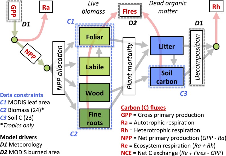
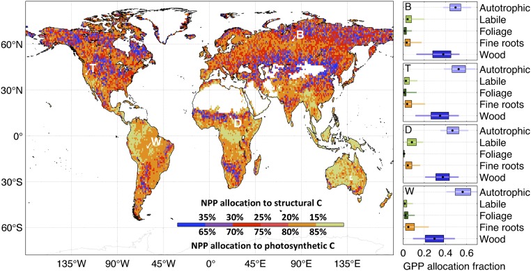
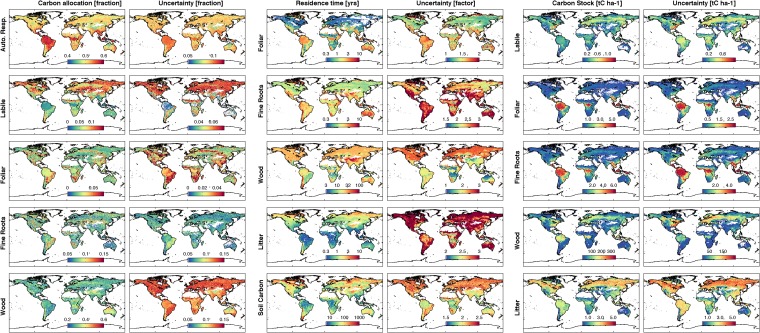
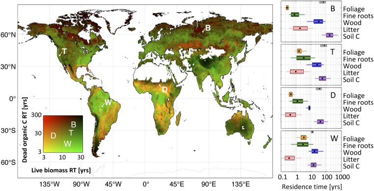
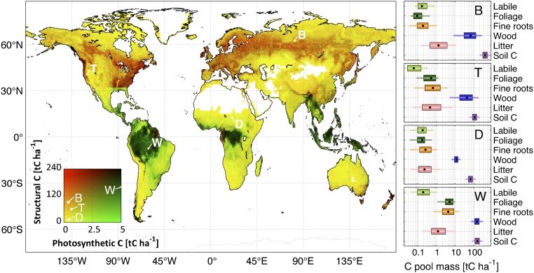
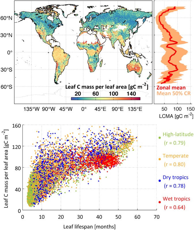
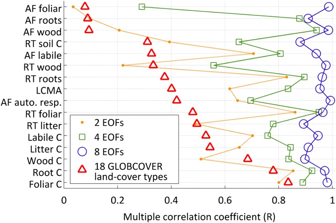
The terrestrial carbon cycle is currently the least constrained component of the global carbon budget. Large uncertainties stem from a poor understanding of plant carbon allocation, stocks, residence times, and carbon use efficiency. Imposing observational constraints on the terrestrial carbon cycle and its processes is, therefore, necessary to better understand its current state and predict its future state. We combine a diagnostic ecosystem carbon model with satellite observations of leaf area and biomass (where and when available) and soil carbon data to retrieve the first global estimates, to our knowledge, of carbon cycle state and process variables at a 1° × 1° resolution; retrieved variables are independent from the plant functional type and steady-state paradigms. Our results reveal global emergent relationships in the spatial distribution of key carbon cycle states and processes. Live biomass and dead organic carbon residence times exhibit contrasting spatial features (r = 0.3). Allocation to structural carbon is highest in the wet tropics (85-88%) in contrast to higher latitudes (73-82%), where allocation shifts toward photosynthetic carbon. Carbon use efficiency is lowest (0.42-0.44) in the wet tropics. We find an emergent global correlation between retrievals of leaf mass per leaf area and leaf lifespan (r = 0.64-0.80) that matches independent trait studies. We show that conventional land cover types cannot adequately describe the spatial variability of key carbon states and processes (multiple correlation median = 0.41). This mismatch has strong implications for the prediction of terrestrial carbon dynamics, which are currently based on globally applied parameters linked to land cover or plant functional types.

Keywords: allocation; biomass; carbon cycle; residence time; soil carbon.

Fig. 1.

Diagnostic ecosystem C balance model DALEC2 (19, 35) and datasets used to retrieve 1° × 1° C state and process variables. GPP, a function of climate and foliar C, is partitioned into autotrophic respiration (Ra) and NPP. NPP is partitioned into the live biomass pools. Plant mortality provides input to the DOM pools. Heterotrophic respiration (Rh) is derived from decomposing DOM pools. Fire fluxes are derived from burned area data (35) and all C pools (SI Text, section S2). Within each 1° × 1° grid cell, we use a Bayesian MDF algorithm to retrieve C state/process variables and uncertainties; variables are retrieved without prior land cover type or steady-state assumptions. Data constraints consist of MODIS leaf area, total biomass (24) (tropics only), and soil C (23). Details on the Bayesian fusion approach are provided in Materials and Methods.

Fig. 2.

Retrievals of NPP allocation to structural (wood and fine roots) and photosynthetic (labile and foliage) C pools. Allocation fractions were retrieved at 1° × 1° using a Bayesian MDF approach (Fig. 1). The GPP allocation fraction retrievals at locations B, T, D, and W are shown on the Right (black dot, median; box, 50% confidence range; line, 90% confidence range).

Fig. S1.

(Left) Posterior GPP C allocation to autotrophic respiration (equivalent to 1 − CUE), labile C, foliar C, fine roots, wood (mean; column 1), and associated uncertainty (SD; column 2). (Center) Posterior C residence time in foliar C; fine roots, wood, litter, and soil C (log-based mean; column 1); and associated uncertainty factors (based on logarithmic SD; column 2). (Right) Posterior mean 2001–2010 C stocks in labile, foliar, fine roots, wood, and litter C pools (mean; column 1) and associated uncertainties (SD; column 2).

Fig. 3.

Retrievals of C residence time (RT) in live biomass and dead organic C pools; residence times are retrieved at 1° × 1° using a Bayesian MDF approach (Fig. 1). Brown denotes ecosystems with high residence times for all C pools, green denotes ecosystems with long live biomass C residence times, and orange denotes ecosystems with low live biomass residence time. The residence times for individual C pools at locations B, T, D, and W are shown on the Right (black dot, median; box, 50% confidence range; line, 90% confidence range). Mean C residence times in ref. are shown as gray boxes (50% confidence intervals) and black dots (medians).

Fig. 4.

Retrieved mean photosynthetic (foliar and labile) and structural (wood and fine roots) C pool stocks; C stocks are retrieved at 1° × 1° using a Bayesian MDF approach (Fig. 1). Retrieved mean C stocks for each pool at locations B, T, D, and W are shown on the Right (black dot, median; box, 50% confidence range; line, 90% confidence range). Dark colors denote high-structural C/high-photosynthetic C ecosystems, green denotes low-structural C/high-photosynthetic C ecosystems, red denotes low-photosynthetic C/high-structural C ecosystems, and yellow denotes low-photosynthetic C/low-structural C ecosystems.

Fig. 5.

(Upper Left) Retrieved median 1° × 1° LCMA (in grams C per meter⁻²). (Upper Right) Zonal mean of median LCMA and 50% confidence range (CR). (Lower) LCMA against leaf lifespan for high latitudes (>55° N/S), temperate regions (23°–55° N/S), dry tropics (precipitation <1,500 mm; <23° N/S), and wet tropics (precipitation >1,500 mm; <23° N/S).

Fig. S2.

CARDAMOM zonal profiles of median GPP, ecosystem respiration, fires, and NCE (red). The 50% confidence range (C.R.) is depicted as a light gray-shaded area. The blue lines represent the eight global MsTMIP models (62) (details in SI Text, section S7). The dashed black line denotes the flux tower-derived GPP (36). The continuous black line denotes the Global Fire Emissions Database version 3 (GFEDv3) total C emissions (36).

Fig. S3.

The 2009–2010 GEOS-Chem model with CARDAMOM mode NCE compared against mean monthly total C column observing network (TCCON) atmospheric column measurements across 12 TCCON sites. Left shows atmospheric CO₂ concentrations, and Right shows the linearly detrended CO₂ anomalies. The detrended comparison Pearson’s r = 0.93, and RMSE = 0.53 ppm. JFM, AMJ, JAS, and OND denote consecutive 3-month periods between January and December.

Fig. S4.

Posterior allocation fractions (alloc), residence times (RT), carbon pools (C), and leaf C mass per leaf area (LCMA) median and 50% confidence ranges shown for 1° × 1° grid cells B, T, D, and W for the unperturbed results (S0) and sensitivity experiments S1–S12. The coordinates of B, T, D, and W are reported in Materials and Methods (locations shown in Inset). Across all locations, 88% of median sensitivity analysis estimates (sensitivity tests S1–S12; SI Text, section S4) are within ±50% of unperturbed median C state and process variable retrievals.

Fig. 6.

Multiple correlation coefficients (R; x axis) of retrieved C state and process variables—allocation fractions (AF), residence times (RT), mean C pools, and LCMA (y axis)—against 18 GLOBCOVER land cover fractions and C variable primary EOFs. R denotes the ability of GLOBCOVER land cover types and primary EOFs to predict 1° × 1° state and process variables (R would equal one if all C state and process variables could be expressed as a linear sum of land cover fractions or EOFs).

Fig. S5.

Maps show eight primary 1° × 1° standardized EOFs 1–8 derived from a principal component analysis of standardized C state and process variables (SI Text, section S6). The two dominant modes (EOFs 1 and 2) together reflect first-order global variations in C state/process variables (c_s) as a result of latitude and precipitation, whereas higher-order modes reflect increasingly complex spatial structures (we note, however, that EOFs 3–8 typically account for a smaller portion of c_s spatial variability). Scatterplots show standardized EOFs 1–8 coefficients corresponding to each C state/process variable (shown as symbol–color combinations). The linear sum of standardized EOFs 1–4 (1–8) and the associated coefficients reproduce 29–95% (88–99%) of C state/process variability (Fig. 6).

Fig. S6.

Pearson’s correlation coefficients (r²; shown in color bar) between GLOBCOVER land cover types fractions (x axis) and C state and process variables—allocation fractions (Alloc), residence times (RT), carbon pools (C), and leaf carbon mass per leaf area (LCMA) (y axis)—based on their correlation across all 1° × 1° grid cells within the global study area. BDF, closed broadleaved deciduous forest; BDFW, open broadleaved deciduous forest/woodland; BESDF, closed to open broadleaved evergreen or semideciduous forest; CRI, irrigated croplands; CRR, rain-fed croplands; FWE, closed to open broadleaved forest regularly flooded; GRA, closed to open herbaceous vegetation; MCV, mosaic cropland > vegetation; MF, closed to open mixed forest; MFSG, mosaic forest or shrub land > grassland; MGFS, mosaic grassland > forest or shrub land; MVC, mosaic vegetation > cropland; NDEF, open needle-leaved deciduous or evergreen forest; NEF, closed (>40%) needle-leaved evergreen forest; SPA, sparse vegetation; SRB, closed to open shrub land; SWE, forest or shrub land permanently flooded; WET, closed to open vegetation on flooded or waterlogged soil.

References

1. Le Quéré C, et al. The global carbon budget 1959–2011. Earth Syst Sci Data. 2013;5(1):165–185.
1. Gatti LV, et al. Drought sensitivity of Amazonian carbon balance revealed by atmospheric measurements. Nature. 2014;506(7486):76–80. - PubMed
1. Dieleman WIJ, et al. Simple additive effects are rare: A quantitative review of plant biomass and soil process responses to combined manipulations of CO2 and temperature. Glob Chang Biol. 2012;18(9):2681–2693. - PubMed
1. Keenan TF, et al. Increase in forest water-use efficiency as atmospheric carbon dioxide concentrations rise. Nature. 2013;499(7458):324–327. - PubMed
1. Reich PB, Hobbie SE. Decade-long soil nitrogen constraint on the CO2 fertilization of plant biomass. Nat Clim Chang. 2013;3(3):278–282.
Publication types
LinkOut - more resources