Topical Review: Molecular reaction and solvation visualized by time-resolved X-ray solution scattering: Structure, dynamics, and their solvent dependence

Abstract

Time-resolved X-ray solution scattering is sensitive to global molecular structure and can track the dynamics of chemical reactions. In this article, we review our recent studies on triiodide ion (I3 (-)) and molecular iodine (I2) in solution. For I3 (-), we elucidated the excitation wavelength-dependent photochemistry and the solvent-dependent ground-state structure. For I2, by combining time-slicing scheme and deconvolution data analysis, we mapped out the progression of geminate recombination and the associated structural change in the solvent cage. With the aid of X-ray free electron lasers, even clearer observation of ultrafast chemical events will be made possible in the near future.

FIG. 1.

Schematic representation of the three principal contributions to the X-ray solution scattering for an I₃^– ion dissolved in water. The I, O, and H atoms are colored in purple, red, and white, respectively. Red arrows indicate atomic pairs of the solute only, while blue and green arrows represent solute–solvent and solvent-only atomic pairs, respectively.

FIG. 2.

(a) Candidate structures of of I₃^– ion in solution. (b) Schematic of candidate reaction pathways for photodissociation of I₃^– ion in solution.

FIG. 3.

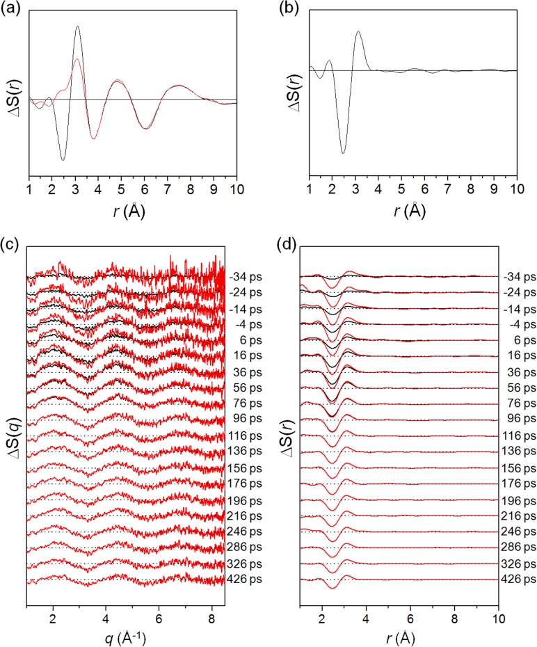
Time-resolved difference X-ray scattering curves of I₃^– ion in methanol measured with ((a), (b)) 400 nm and ((c), (d)) 267 nm laser excitation. (a) Experimental difference scattering curves, qΔS(q,t), measured with 400 nm laser excitation (black) and their theoretical fits (red) are shown together. (b) Corresponding difference radial distribution functions, rΔS(r,t), obtained by sine-Fourier transformation of qΔS(q,t) in (a). (c) Experimental difference scattering curves, qΔS(q,t), measured with 267 nm laser excitation (black) and their theoretical fits (red) are shown together. (d) Corresponding difference radial distribution functions, rΔS(r,t), obtained by sine-Fourier transformation of qΔS(q,t) in (c).

FIG. 4.

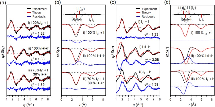
Determination of the reaction pathways of I₃^– photodissociation in methanol with ((a), (b)) 400 nm and ((c), (d)) 267 nm laser excitations in ((a), (c)) q-space and ((b), (d)) r-space. (a) Theoretical difference scattering curve (red) for each candidate pathway is shown together with the experimental difference scattering curve at 100 ps (black). The model employing only the two-body dissociation pathway gives much better fit than the models employing the three-body dissociation and I₂ formation pathways, indicating that two-body dissociation is the dominant reaction pathway with 400 nm laser excitation. (b) Radial distribution functions, rΔS(r,t), of solute-only term. Bond distances and their contributions of various I–I pairs are indicated as red bars and dashed curves, respectively, at the top. With the model employing only two-body dissociation, the experimental and theoretical RDFs of solute-only term are in good agreement. (c) The same analysis of (a) for 267 nm laser excitation. The models employing the two-body and three-body dissociation pathways give similarly good fitting qualities, indicating the possibility of multiple reaction pathways. The best fit was obtained with a model employing all three reaction pathways. The optimum ratio of the contributions of two-body and three-body dissociation was determined to be 7:3. (d) The same analysis of (b) for 267 nm laser excitation. With the model employing the two-body and three-body dissociation pathways with the branching ratio of 7:3, the experimental and theoretical PDFs of solute-only terms are in good agreement.

FIG. 5.

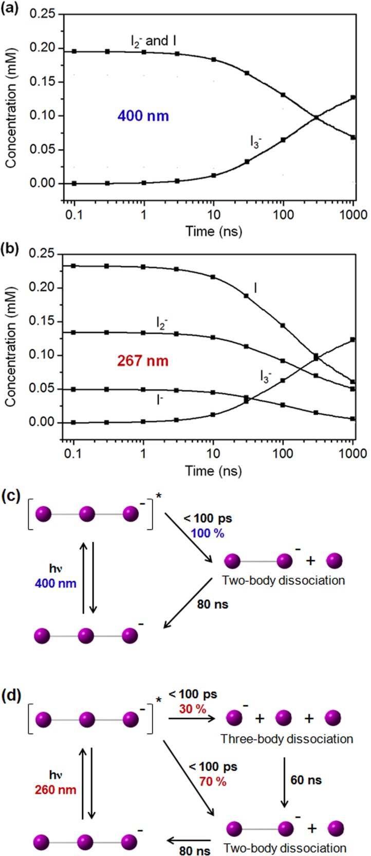
(a) Time-dependent concentration changes of various transient solute species after photodissociation of I₃^– ion in methanol with 400 nm excitation. (b) Time-dependent concentration changes of various transient solute species after photodissociation of I₃^– ion in methanol with 267 nm excitation. (c) Reaction mechanism of I₃^– photodissociation at 400 nm. (d) Reaction mechanism of I₃^– photodissociation at 267 nm.

FIG. 6.

(a) Atom-atom pairs probed by static X-ray solution scattering. Since X-rays scatter off from every atom in the solution, the scattering pattern is very complicated. (b) Scattering intensity of I₃^– ion extracted from static wide-angle X-ray solution scattering (black). Scattering patterns from pure solvent and air as well as the dark response of the detector were subtracted from the scattering pattern of the solution sample. The theoretical scattering curve (red) does not match the experimental difference curve due to the unknown background remaining. Therefore, we cannot obtain the exact structure of I₃^– ion within a reasonable error range.

FIG. 7.

Schematic of (a) our experimental approach using TRXSS experiment and (b) data analysis. Upon irradiation at 400 nm, I₃^– ion dissociates into I₂^– and I, and the temperature of the solution increases. By taking the difference between scattering patterns measured before and 100 ps after laser excitation, only the laser-induced changes are extracted with all other background contributions being eliminated. The structural information can be extracted by the maximum likelihood estimation using five fitting parameters. Three bond distances of I₃^– can be clearly identified, giving the exact structure of I₃^– ion in various solvents.

FIG. 8.

Difference scattering curves measured at 100 ps after photoexcitation for the I₃^– photolysis in water, acetonitrile, and methanol solution. Experimental (black) and theoretical (red) curves using various candidate structures of I₃^– ion are compared. Residuals (blue) obtained by subtracting the theoretical curve from the experimental one are displayed at the bottom. (a) In water, I₃^– ion was found to have an asymmetric and bent structure. To emphasize the fine difference in fitting quality, the residuals shown were multiplied by a factor of 3. (b) In acetonitrile, I₃^– ion was found to have a symmetric and linear structure. (c) In methanol, I₃^– ion was found to have an asymmetric and linear structure.

FIG. 9.

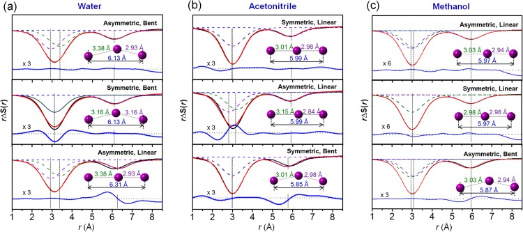
Structure reconstruction of I₃^– ion based on the extracted bond distances. The contribution of I₃^– alone (black solid line) was extracted. Theoretical curves (red) were generated by a sum of three I–I distances (dashed lines). The residuals (blue solid line) are displayed at the bottom. (a) In water solution, the theoretical curve calculated from the asymmetric and bent structure gave the best fit to the experimental curve (top panel). When one average distance (3.16 Å) instead of two unequal distances was used, the broad feature in the experimental curve cannot be matched (middle panel). When a linear and asymmetric structure is used, the sum of two I–I distances (6.31 Å) do not match the R₃ (6.13 Å) determined from the experimental scattering curve, indicating the bent structure (bottom panel). (b) In acetonitrile solution, a symmetric and linear structure gave the best fit (top panel). If two unequal distances (3.15 Å and 2.84 Å) were used, the theoretical curve becomes broader than the experimental curve (middle panel). When a bent structure was used, the peak at 5.99 Å is shifted to a smaller value, giving a worse fit to the experimental curve (bottom). (c) In methanol solution, a symmetric and linear structure gave the best fit (top panel). If two equal distances were used, the theoretical curve becomes slightly narrower than the experimental curve (middle panel). When a bent structure was used, the peak at 5.97 Å is shifted to a smaller value, giving a worse fit to the experimental curve (bottom).

FIG. 10.

Optimized structures and the relative energies of I₃^– ion with 34 explicit water molecules forming the first solvation shell by DFT method. The optimized structure of I₃^– ion has a broken symmetry (asymmetric, bent) and is stabilized by 51.2 kJ/mol compared with the linear symmetric one. The elongated iodine atom has more negative charge than the other iodine atom, resulting in stronger interaction with surrounding hydrogen atoms of water molecules.

FIG. 11.

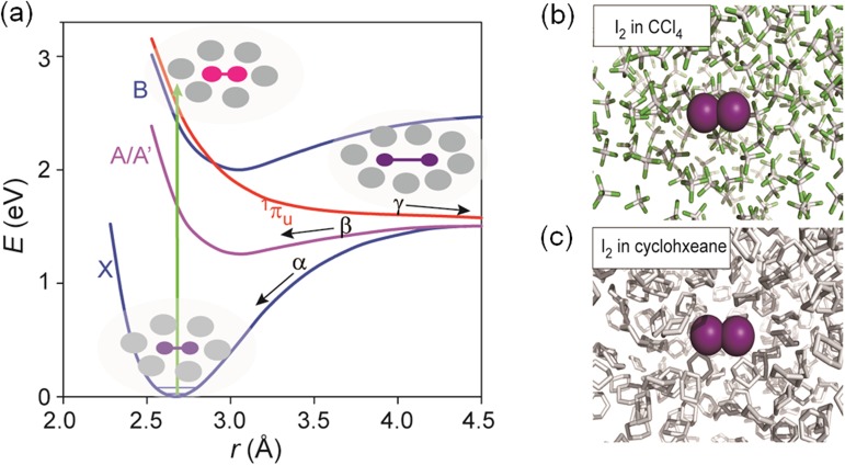
(a) Potential energy surface of I₂ in CCl₄. Low-lying electronic states (X, A/A′, B and ¹π_u) of I₂. The states A and A′ are closely spaced and can be viewed as a single electronic state A/A′. The processes α and β represent geminate recombination of two I atoms in the X and A/A′ states, respectively. The process γ represents nongeminate recombination through the solvent. Schematic snapshots of solute-solvent configuration at representative stages are depicted. (b) MD snapshot of I₂ in CCl₄. Purple sphere is iodine atom, grey rod is carbon atom, and green is chloride atom. (c) MD snapshot of I₂ in cyclohexane. Purple sphere is iodine atom, and grey rod is carbon atom.

FIG. 12.

Schematic of the time-slicing experiment. At a negative time delay (e.g., −30 ps) close to time zero, the X-ray pulse arrives (effectively) earlier than laser pulse, but the X-ray pulse, which is much longer in time than the laser pulse, is still present after the interaction with the laser pulse and thus scattered off the laser-illuminated sample. At time zero, half of the X-ray pulse probes the laser-illuminated sample. At a positive time delay, most of the X-ray pulse is scattered off the laser-illuminated sample.

FIG. 13.

Difference scattering curves for solute and solvent-only contributions. (a) ΔS(r,426 ps) curve from I₂/CCl₄ solution (black) and ΔS(r,200 ps)_solvent-only curve from thermally excited CCl₄ (red). (b) Solute-related ΔS(r,426 ps) obtained by subtracting the solvent contribution from the solution signal. Note the negative peak arising from the depletion of I₂ in the ground (X) state and the positive peak corresponding to the A/A′ state. (c) Solute-related ΔS(q, t) curves with the solvent contribution eliminated. At early times, only a fraction of the X-ray pulse probes the laser-triggered molecules and thus the amplitudes of raw difference scattering signals at early times (black curves) are small. Considering the effect of this partial temporal overlap, the difference scattering curves at early times were scaled up (red curves) following the temporal rise of the signal in the form of an error function. (d) Solute-related ΔS(r, t) curves obtained by Fourier transform of the curves shown in (c). Note that the depth of the negative peak at 2.6 Å decreases with time as the geminate recombination progresses and leads to recovery of I₂ in the ground state.

FIG. 14.

(a) The spectrum of X-ray pulse used in the experiment has a 3% bandwidth and a characteristic half-Gaussian shape. (b) A scheme for correcting the effect of polychromatic X-ray spectrum on the difference scattering curve. The polychromaticity of the X-ray spectrum induces the shift of ΔS(r) along r-axis (red curve). The black curve is a trial scattering curve obtained with a monochromatic X-ray beam. When the trial scattering curve is convoluted with the polychromatic spectrum, a blue curve is generated. By fitting the experimental data (red curve) with the convoluted trial curve (blue curve) using least-squares refinement of the trial curve, we can obtain ΔS[r] under monochromatic conditions.

FIG. 15.

(a) Concept of deconvolution. If the temporal duration of X-ray pulse is larger or comparable to the time scale of the process of interest, the dynamic features become blurred in the experimental data due to the convolution of the sample signal with the temporal profile of the X-ray pulse. Upper figure shows r²ΔS(r,t) with respect to time at r = 3.1 Å. For each r value, r²ΔS(r,t) results from the convolution of the sample signal r²ΔS_inst(r,t) with the X-ray temporal profile I_x-ray(t). The goal of deconvolution is to reconstruct r²ΔS_inst(r,t) from r²ΔS(r,t). (b) Time-dependent deconvoluted difference scattering curves r²ΔS_inst(r,t) for I₂ in CCl₄. (c) The same analysis for I₂ in cyclohexane.

FIG. 16.

(a) r²ΔΔS_inst(r,t) for I₂ in CCl₄ obtained by subtracting r²ΔS_inst(r,426 ps) from r²ΔS_inst(r,t) to remove the contribution from the A/A′ state and dissociated iodine atoms remaining at 426 ps. (b) r²ΔΔS_inst(r,t) for I₂ in CCl₄ obtained by subtracting the contribution from the population decay of A/A′ (1.2 ns).

FIG. 17.

(a) Time-dependent I–I distance distribution functions, r²S_inst(r,t), of I₂ in CCl₄. (b) Cross sections of r²S_inst(r,t) at the time delays indicated by dotted lines in (a). (c) ⟨r(t)⟩ was calculated from (a) and compared with a single exponential fit (blue) and a double exponential fit (red). To obtain a satisfactory fit to the experimental data, a double exponential is necessary with the time constants of 16 ps and 76 ps and a relative amplitude ratio of about 2:1. (d) Time evolution of the I–I distance distribution function, r²S_inst(r,t) (blue, solid line), converted from ρ(r,t) of the I–I atomic pair obtained from MD simulation (black, dotted line). The potential energy curve corresponding to the X state is also shown (red, dashed line). (e) Time dependence of the average I–I distance, ⟨r⟩, calculated from the I–I distance distribution function, r²S(r,t). Fit of the average distance ⟨r⟩ (blue, solid line) by a double exponential function, g(t) = A_r exp(−t/τ₁^r) + B_r exp(−t/τ₂^r) + 2.67 Å (red, dashed line), gives the relaxation times τ₁^r = 3 ps and τ₂^r = 44 ps. The equilibrium distance (green, dash-dotted line) is also shown.

FIG. 18.

(a) Time-dependent I–I distance distribution functions, r²S_inst(r,t), of I₂ in cyclohexane. (b) Cross sections of r²S_inst(r,t) at the time delays indicated by dotted lines in (a). (c) ⟨r(t)⟩ was calculated from (a) and fit by a single exponential fit (red). The single exponential gives a satisfactory fit to the experimental data with a time constant of 55 ps.

FIG. 19.

(a) Experimental r²ΔS_inst(r,t) curves at large r values corresponding to time-dependent solute–solvent (mostly I–Cl) distance distribution functions, r²ΔS_cage(r,t). (b) Theoretical time-dependent solute–solvent distance distribution functions, r²ΔS_cage(r,t), based on the experimentally obtained I–I distribution (shown in Figure 17(a)) and the solute-solvent atom–atom pair distribution functions, g(r), calculated by MD simulation. (c) Interatomic pair distribution functions between a C atom of the solvent and an I atom of the solute, g_C–I(r). The red and blue curves are for the solute with the I–I distance of 4.0 Å and 3.1 Å, respectively, and the black curve is for the solute with the I–I distance of 2.65 Å. (d) Interatomic pair distribution functions between a Cl atom of the solvent and an I atom of the solute, g_Cl–I(r). The red and blue curves are for the solute with the I–I distance of 4.0 Å and 3.1 Å, respectively, and the black curve is for the solute with the I–I distance of 2.65 Å. (e) Theoretical solute–solvent distance distribution function, r²_cageS(r), is obtained from g(r) – 1 calculated from MD simulation. (f) Theoretical difference cage term r²ΔS_cage(r) is obtained by subtracting r²S_cage(r) of I₂ in the ground-state configuration from r²S_cage(r) of I₂ with the I–I distance in the range of 2.3 – 4.2 Å. With the decrease of I–I distance towards the equilibrium distance in the ground state, the width of negative peak at around 6 Å is narrowed, and positive peak between 7 and 8 Å is shifted to 7 Å.

FIG. 20.

(a) and (b) Examples of the difference Cl–I pair distribution functions, Δg_Cl–I(r), and the difference C–I pair distribution functions, Δg_C–I(r), obtained from the MD simulation. The blue and red curves are for I–I distance changes from 2.65 Å to 4.0 Å and 2.65 Å to 3.1 Å, respectively. (c) Schematic for the change of the solvation shell due to the elongation of I–I distance. Dotted circles indicate the first solvation shell. The interatomic distance shown in this figure is the distance between the I atom of the solute and the C atom in the solvation shell. Because a CCl₄ molecule has one C atom surrounded by four Cl atoms and the Cl atom scatters much more strongly than the C atom, the scattering signal is dominated by the I−Cl contribution. Nevertheless, with the C atom being located at the center of the CCl₄ molecule, the I−C distribution provides a more intuitive picture of the size of the solvation shell.

FIG. 21.

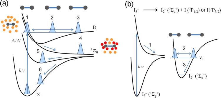
(a) Photodissociation dynamics of I₂ in solution phase. Upon photoexcitation by an optical pulse, coherent vibrational wave packet evolves in the B state to induce the periodic oscillation of I–I bond length (1, 2, and 3). Subsequently, the excited population relaxes to a repulsive ¹π_u state, leading to either dissociation of I₂ (4) or geminate recombination via A/A′ state (5) or hot ground state (6). (b) Photodissociation dynamics of I₃^– ion. Upon photoexcitation of I₃^– by an optical pulse, one I atom is dissociated (1), forming coherent vibrational wave packet in the hot ground state (²Σ_u⁺) of I₂^–. As the coherent wave packet evolves in the hot ground state of I₂^– ion, the I–I bond length of the I₂^– ion periodically oscillates (2). Subsequently, the population in the hot ground state of I₂^– relaxes vibrationally to the ground state of I₂^– (3).