The temporal scaling of Caenorhabditis elegans ageing

Abstract

The process of ageing makes death increasingly likely, involving a random aspect that produces a wide distribution of lifespan even in homogeneous populations. The study of this stochastic behaviour may link molecular mechanisms to the ageing process that determines lifespan. Here, by collecting high-precision mortality statistics from large populations, we observe that interventions as diverse as changes in diet, temperature, exposure to oxidative stress, and disruption of genes including the heat shock factor hsf-1, the hypoxia-inducible factor hif-1, and the insulin/IGF-1 pathway components daf-2, age-1, and daf-16 all alter lifespan distributions by an apparent stretching or shrinking of time. To produce such temporal scaling, each intervention must alter to the same extent throughout adult life all physiological determinants of the risk of death. Organismic ageing in Caenorhabditis elegans therefore appears to involve aspects of physiology that respond in concert to a diverse set of interventions. In this way, temporal scaling identifies a novel state variable, r(t), that governs the risk of death and whose average decay dynamics involves a single effective rate constant of ageing, kr. Interventions that produce temporal scaling influence lifespan exclusively by altering kr. Such interventions, when applied transiently even in early adulthood, temporarily alter kr with an attendant transient increase or decrease in the rate of change in r and a permanent effect on remaining lifespan. The existence of an organismal ageing dynamics that is invariant across genetic and environmental contexts provides the basis for a new, quantitative framework for evaluating the manner and extent to which specific molecular processes contribute to the aspect of ageing that determines lifespan.

Extended Data Figure 1. Characterizing the shape of wild-type lifespan distributions at 20 °C

a, The AFT residuals corresponding to the 20 °C wild-type population presented in Fig. 1 were fitted with a variety of parametric distributions (Supplementary Note 1.4). Fits made to AFT residuals, as opposed to absolute death times, are much less sensitive to any environmental heterogeneity existing between plates and scanners (Statistical methods). b, The AFT residuals of four additional replicates at 20 °C to assess deviations from temporal scaling between replicates. c, The Akaike information criterion (AIC) was calculated for the each parametric fit of each replicate’s AFT residuals shown in panel b. Lower AIC values suggest preferred models. d, The parameters of Gompertz and Weibull distributions with frailty corrections are listed; both distributions were good fits across all replicates. e, f, The survival curves of populations collected in two biological replicates are shown, with one curve for individuals observed on each of 10 and 6 scanners respectively. g, The modified Kolmogorov–Smirnov Y(t) (Supplementary Note 2) is plotted for comparisons between replicate 1 and all others. Pairs for which Y(t) > 1.51 for some t exhibit statistically significant deviations from perfect scaling. In this case every replicate differed significantly from the first replicate. h, The distribution of modified Kolmogorov–Smirnov score scores, Ῡ, is plotted for comparisons between scanners within a replicate (blue) and between scanners in different replicates (red). Differences between replicates were larger than differences with replicates, suggesting that distance between survival curves observed between scanners cannot alone explain the distance between survival curves observed between replicates. i, The P values corresponding to each Ῡ are shown, with values P > 0.01 considered statistically significant (grey line).

Extended Data Figure 2. Apparent deviations from temporal scaling are observed when single replicates are performed at each temperature

a, For the data shown in Fig. 1a, the modified Kolmogorov–Smirnov test Y(t) was calculated for AFT residuals (Statistical methods and Supplementary Note 2) to compare the reference population at 20 °C with populations held at each of the other temperatures. Pairs for which Y(t) > 1.51 for some t (grey dashed line) exhibit significant deviations from perfect scaling. b, The modified Kolmogorov–Smirnov test scores Ῡ, corresponding to the maximum absolute value of Y(t) observed at any time t, are shown for the comparisons in a, highlighting the statistical deviations observed between independent replicates performed at different temperatures. c, d, The same statistics were calculated when comparing all populations above 30 °C with the population at 30 °C.

Extended Data Figure 3. Independent replicates demonstrate that apparent deviations from temporal scaling within low- and high-temperature regimes arise from uncontrolled environmental variation

The lifespan of individuals from populations housed between 20 °C and 34 °C were collected using the lifespan machine (also shown in Fig. 4a, b). To characterize the effects of any uncontrolled experimental conditions specific to individual replicates, and identify any effects of temperature consistent across replicates, we divided the full temperature range into 2 °C intervals. Each 2 °C interval contained lifespan data collected in either two or three independent replicate experiments performed in separate weeks. a, Within each 2 °C range, all death times were fitted by an AFT regression model using plate name as a categorical covariate (Statistical methods). The device-corrected death times (the residual time plus model intercept) were plotted, highlighting the changes in survival curve shape between replicates within each 2 °C range. b, All deaths across all temperatures were then fitted by a single AFT regression model with plate name as the categorical covariate. AFT residuals were grouped according to their replicate name and temperature range, and plotted to highlight the deviations from temporal scaling across all replicates at all temperatures. c, The modified Kolmogorov–Smirnov test (Supplementary Note 2) was applied on each pair of curves shown in b. The resulting Kolmogorov–Smirnov Ῡ was used as a distance metric with which to perform a hierarchical clustering, shown as a dendrogram with each replicate population labelled by the temperature at which it lived. In this dendogram, populations exhibiting smaller deviations from temporal scaling will have fewer branches between them. Clades that contain statistically significant deviations from temporal scaling have branches extending beyond the dashed grey line, indicating that Ῡ > 1.51 between branches. Six statistically distinct groups were identified, three above 30 °C and three below. d, The same dendogram is shown with populations labelled according to the name of the replicate in which they were collected. Populations collected in single replicates did not fall into single clades. This suggests that some environmental factor variable within replicates, distinct from the particular temperature at which populations were placed, produced the observed deviations from temporal scaling. e, The statistically distinct clades identified by hierarchical clustering (c) are plotted on a temperature scale. Clades overlap at all temperatures except the 30 °C boundary, suggesting that only the 30 °C transition represents a true temperature-dependent deviation from temporal scaling. f, The aggregate survival curves containing the AFT residuals of all individuals in each statistically distinct clade are compared, to highlight the differences in shape between clades. g, The hazard rate plot of the AFT residuals of all individuals in each statistically distinct clade. h, Break out of the hazards for only for low-temperature populations. i, Break out of the hazards for only high-temperature populations.

Extended Data Figure 4. Additional survival curves and hazard plots

a, The hazard rates corresponding to the tBuOOH survival data presented in Fig. 1: 0 mM (black), 1.5 mM (blue), 3 mM (green), and 6 mM (red). b, To test for any effects of tBuOOH degradation and evaporation on lifespan, 9 mM tBuOOH plates were prepared and placed at 4 °C. On 4 consecutive days, a subset of plates were seeded with ultraviolet-inactivated bacteria and placed without C. elegans on scanners operating at 20 °C. In this way, four groups of plates were created, corresponding to 0, 1, 2, and 3 days of cumulative exposure to standard scanner conditions during which tBuOOH degradation and evaporation could potentially occur. A single age-synchronous population of 2-day-old adult C. elegans was then simultaneously distributed across all plates. The remaining lifespan of all worms at 20 °C was recorded using the lifespan machine. c, In a separate experiment, plates were prepared containing either 3 mM tBuOOH or 3 mM t-butanol, a degradation product of tBuOOH. On t-butanol, only a trivial fraction of individuals had died by the fifth day, so the experiment was terminated. d, e, The survival of wild-type and age-1(hx546) populations at 25 °C. f, g, The lifespan and AFT residuals for hif-1(ia4) and wild-type populations, calculated as in Fig. 2. h, i, The lifespan and AFT residuals for eat-2(ad1116) at 20 ° and 22.5 °C. j–o, Age-synchronous mutant (red) and wild-type (black) populations were raised at 25 °C and then transferred to 33 °C on their second day of adulthood, where they remained until death. For each population at 33 °C, the hazard rate was estimated from the death times (j, l, n). The hazard rate was also estimated from the residuals of the AFT regression model log(y_i) = βx_i + ε_i with genotype as a single categorical covariate (k, m, o). p, q, The hazard functions of death times and AFT residuals corresponding to the daf-16(mu86) data presented in Fig. 1. r, s, The hazard functions of death times and AFT residuals corresponding to the daf-2(1368) data presented in Fig. 1. t, u, The hazard functions of death times and AFT residuals corresponding to the eat-2(ad1116) data presented in Fig. 1. v, w, The hazard functions of death times and AFT residuals corresponding to the nuo-6(qm200) data presented in Fig. 1.

Extended Data Figure 5. Additional temperature shift data

a, As a control for the temperature shift experiment shown in Fig. 3, the same regression as in Fig. 3c was run to test for temporal scaling between populations always held at 24 °C (black) and those always held at 29 °C (red). The residuals ε_i are plotted as hazard functions. b, The same regression as in Fig. 3 was run for the same populations as b here, to test for temporal shifts. c, To test for the effects of different durations spent at 24 °C before transfer to 29 °C. Age-synchronous, wild-type animals were grown at 20 °C and then transferred on their second day of adulthood to 24 °C. Subsets of these animals were then transferred to 29 °C on each of 3 consecutive days. d, For each population, the remaining lifespan was observed and the hazard functions estimated. All death times represent the number of days after the second day of adulthood. e, The residuals from a regression model with the duration at 24 °C as an additive categorical covariate y_i = βx_i + ε_i. f, The residuals from a regression model with the duration at 24 °C as a proportional covariate log(y_i) = βx_i + ε_i. g, The shift values β=Δ_τ of the additive model are plotted along with a linear fit. h, To test for the effect of rapid temperature changes on lifespan, age-synchronous individuals were raised at 20 °C. On their second day of adulthood, a subset was transferred to 29 °C. i, Another subset of individuals remained at 24 °C for 2 days, after which they were transferred to 29 °C. j, Another subset was transferred to 29 °C, but switched down from 29 °C to 24 °C and then back again to 29 °C (filled circle; three shifts). k, A final subset was switched down and back twice (filled circle; five shifts). Note that all populations spent the same total duration at 29 °C, except for the aforementioned control population that was never switched. l, The data were fitted with an additive regression model y_i = βx_i + ε_i with the number of switchings as a categorical covariate. The encoding of this covariate was set so that all β=Δ_τ represent each subpopulation’s change in lifespan relative to the control population that was never switched.

Extended Data Figure 6. Identifying the number of thermal regimes, and the boundaries between them

The thermal scaling data presented in Fig. 4a were fitted with a segmented regression model (Statistical methods) assuming that λ⁻¹ relates to temperature either following an Arrhenius relationship, λ⁻¹(T) = p₀ exp(p₁/RT) (a, c, e, g, i, k) or a linear relationship, λ⁻¹ (T) = p₀ T + p₁ (b, d, f, h, j, l; Statistical methods). The model fits are plotted in black, with model breakpoints shown as vertical lines. Colours correspond to independent replicates. Each model was fitted assuming a single segment (a, b), two segments (c, d), three segments (e, f), four segments (g, h), five segments (i, j), or six segments (k, l). m, The AIC corresponding to each number of segments for the Arrhenius is plotted. n, The AIC for the linear model is plotted. Because the the Arrhenius and linear models models are fit to distinct data sets (log-transformed and untransformed scale factors respectively, and inverse temperature and untransformed temperatures, respectively), AIC values cannot be compared between Arrhenius and inverse time models. Regime I can be adequately described either by one linear regime or two piecewise Arrhenius regimes, Ia and Ib. Across multiple replicates, the linear 1/T model consistently underestimated C. elegans lifespan around 25 °C, leading us to favour the piecewise Arrhenius model (See Extended Data Figure 6). Regimes II and III involve temperature ranges that are too narrow to distinguish between Arrhenius and linear models. Above 35.5 °C, lifespan is too short to be accurately measured with our time-lapse technique.

Extended Data Figure 7. Additional data for the regression models in Fig. 4b, d

The residuals of the linear model (a) shown in Extended Data Fig. 6f. The residuals of the Arrhenius Arrhenius model (b) shown in Fig. 4b are depicted, showing the deviation of the predicted value from the empirical data across each regime. Residuals are presented in the form of relative error, the ratio between the model’s prediction and the empirical measurement. c, As in Fig. 4d, the response of each genotype, wild type (black), daf-16(mu86) (red), daf-2(e1368) (green), and age-1(hx546) (blue) to changes of temperature was estimated (Statistical methods) in regime II and in regime III.

Extended Data Figure 8. The potential effects of heterogeneity at 33 °C

a, Fifty-six thousand samples were drawn from the distribution of frailty effects Z^−1/α as described in Supplementary Note 3.1, where Z is a random variable, sampled from an inverse-gamma distribution with mean 1 and a standard deviation corresponding to the value estimated from experimental data. Samples were drawn using the σ² estimated for populations at 25 °C (black) and at 33 °C (red), corresponding to the data presented in Fig. 1d. The probability density function of each population is shown, which can be interpreted as the variable effect of unknown factors on lifespan across individuals at each temperature. b, At each temperature, 25 °C (black) and at 33 °C (red), we estimated the distribution of temperature changes required to produce the distribution of frailties shown in a. This was accomplished using temperature scaling function shown in Fig. 4b. c, Fifty-six thousand random samples were drawn from the transformed inverse gamma distribution of Z^−1/α with σ² set to the estimate of Δσ² in equation (15) of Supplementary Note 3.2. Each sample was multiplied by a death time drawn (with replacement) from the set of 25 °C residual times of Fig. 1d, shown here in black. These products constitute a ‘transformed’ set of death times, corresponding to the 25 °C residuals with additional frailty synthetically introduced. The residual death times of animals placed at 33 °C are shown for comparison (red).

Extended Data Figure 9. The organization of lifespan determinants (schematic)

a, A set of molecular determinants of risk of death (open circles) do not interact, as is assumed in a competing risks and weakest link models. b, Risk determinants might interact (arrows) in complex ways to determine lifespan. In this schematic, each risk of death is still determined by separate factors. c, Our data on temporal scaling suggest that the set of molecular determinants that determine risk of death (within the dotted circle) must change in concert when exposed to interventions in ageing. This set is therefore well described by a single state variable r. d, A cartoon of the stochastic decline of such a state variable (generated from the dependency model discussed in Supplementary Note 5.2). Each trajectory represents the values of r over time for each individual in a population. Interventions affect the dynamics of the state decline by rescaling the average dynamics of exposed individuals (red lines), which produces (e) a rescaling of the resultant survival curve. f, Transient interventions in young adults (applied within the red dotted vertical lines) transiently rescale the average dynamics, leading to (g) a shift in the lifespan distribution.

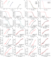
Figure 1. Environmental determinants rescale C. elegans lifespan distributions

a, Populations grown at 20 °C were transferred on their second day of adulthood to a final temperature of (right to left) 20.1 °C (black), 23.7, 25.2, 29.1, 30, 30.9, 31.3, 32.5, and 32.6 (yellow). Individual lifespans were collected and used to estimate the hazard function of each population using numerical differentiation of the Kaplan–Meier survival estimator (solid lines). The shaded areas represent the 95% confidence bands of the true hazard (Statistical methods). b, The lifespan of individuals living at 20, 25, 27, and 33 °C. c, The data in b were fitted with an AFT model log(y_i) = βx_i + ε_i to remove differences in timescale (Methods and Supplementary Note 1.3). The AFT residuals exp(ε_i) corresponding to populations at 20, 25, and 27 °C are plotted using the Kaplan–Meier survival estimator. d, The AFT residuals corresponding to populations held at 25 (black) and 33 °C (red) are plotted using the Kaplan–Meier survival estimator. e, Hazard functions were estimated from the 25 and 33 °C AFT residuals. f, The survival curves of populations exposed to 0 (black), 1.5 (blue), 3 (green), and 6 mM (red) tBuOOH. g, The AFT residuals for the data of f. h, The survival curves of animals cultured on live E. coli (black) and ultraviolet-inactivated E. coli (green). i, The AFT residuals for the data of h.

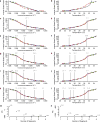
Figure 2. Genetic determinants rescale C. elegans lifespan distributions

Survival curves are shown for (a) daf-2(e1368) (red) and wild type (black) at 25 °C, (b) daf-16(mu86) (red) and wild type (black) at 25 °C, and (c) hsf-1(sy441) (red) and wild type (black) at 20 °C. d–f, The AFT residuals corresponding to the data in a–c respectively. Survival curves are shown for (g) eat-2(ad1116) (red) and wild type (black) at 20 °C, (h) nuo-6(qm200) (red) and wild type (black) at 25 °C, and (i) nuo-6(qm200) populations held at 20 °C and 25 °C. j–l, The AFT residuals corresponding to the data in g–i respectively.

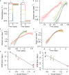
Figure 3. Transient interventions during early adulthood shift the lifespan distribution

a, A schematic: populations were placed at 24 °C (blue), 26 °C (green), 27.5 °C (orange), and 29 °C (red). After τ = 3.2 days, sub-populations were transferred to either 24 °C or 29 °C for the remainder of their lives. b, The hazard rate was estimated using the remaining lifespan of populations transferred to the final temperature of 29 °C. c, To test for temporal scaling between the populations shown in b, death times were fitted with the regression model log(y_i) = βx_i + ε_i, in which exp(β_i) is the best estimate for the scale factor λ. The residuals exp(ε_i) are plotted as hazard functions in the colour scheme of a. d, To test for temporal shifts between the populations shown in b, death times were fitted with the regression model y_i = βx_i + ε_i, in which β_i is the best estimate for the shift term Δ_τ. The residuals ε_i are plotted as hazard functions in the colour scheme of a. e, The shift term Δ_τ for populations transferred from each high temperature to 24 °C was plotted against 1 – λ⁻¹, where λ is the scale factor relating populations always held at the corresponding high temperature to those always held at 24 °C. The prediction Δ_τ = τ(1 – λ⁻¹) suggests that these points should fall along a line with a slope equal to τ in a. A linear regression on these points model estimates τ = 3.38 ± 0.17. f, As in e, but for populations transferred from lower initial temperatures to the final higher temperature of 29 °C, producing the estimate τ = 3.16 ± 0.14.

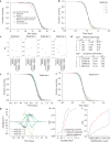
Figure 4. Scaling functions

a, The magnitude of temporal scaling was estimated for wild-type populations held at fractional degree intervals across the range 20–35 °C. The scale factor λ of each population was estimated relative to a reference population at 25 °C. Grey lines mark the average lifespan of the reference population scaled by λ. Each replicate is shown as a separate colour, with each point corresponding to an aggregate population consisting of on average 130 individuals at the outset. b, The scale factor λ was determined for populations across the temperature range of a. The data points were fitted with a segmented Arrhenius model λ⁻¹(T) = p₀ exp(p₁/RT) (red). c, The magnitude of scaling produced by daf-16(mu86) (red), daf-2(e1368) (green), and age-1(hx546) (blue) alleles relative to wild type was estimated at each temperature considered (points). Solid curves represent trends across temperature as fitted by a Loess regression. d, The combined magnitude of scaling produced by each allele and change of temperature was estimated relative to a single wild-type population 24 °C; colours as in c. Regimes II and III are shown in Extended Data Fig. 7. e, Wild-type populations at 20 °C were exposed to a series of tBuOOH concentrations ranging from 0 to 10 mM. For each population, λ was calculated relative to an unexposed population (0 mM). Data for concentrations above 0.75 mM were fitted by the model λ ([tBuOOH]) = p₂([tBuOOH])^p3 (red), yielding p₂ = 0.47 ± 0.02 and p₃ = −1.86 ± 0.15. f, As in c, but for the tBuOOH dosage series.

References

1. Pincus Z, Smith-Vikos T, Slack FJ. MicroRNA predictors of longevity in Caenorhabditis elegans. PLoS Genet. 2011;7:e1002306. - PMC - PubMed
1. Herndon LA, et al. Stochastic and genetic factors influence tissue-specific decline in ageing C. elegans. Nature. 2002;419:808–814. - PubMed
1. Shaw RF, Bercaw BL. Temperature and life-span in poikilothermous animals. Nature. 1962;196:454–457. - PubMed
1. Mair W, Goymer P, Pletcher SD, Partridge L. Demography of dietary restriction and death in Drosophila. Science. 2003;301:1731–1733. - PubMed
1. Wu D, Rea SL, Cypser JR, Johnson TE. Mortality shifts in Caenorhabditis elegans: remembrance of conditions past. Aging Cell. 2009;8:666–675. - PMC - PubMed
Publication types