Neural Mechanisms of Credit Assignment in a Multicue Environment

Abstract

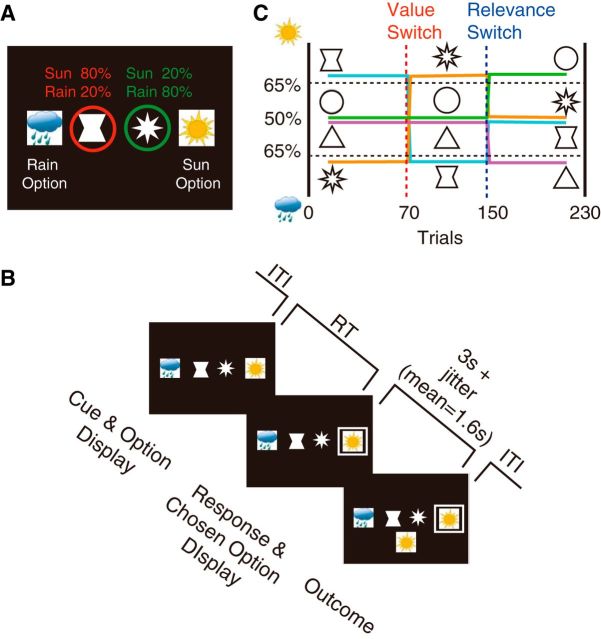
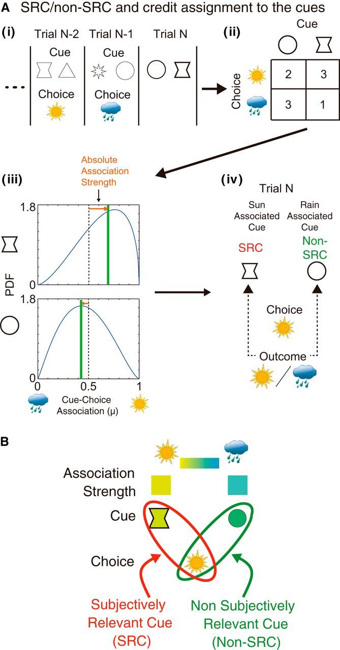
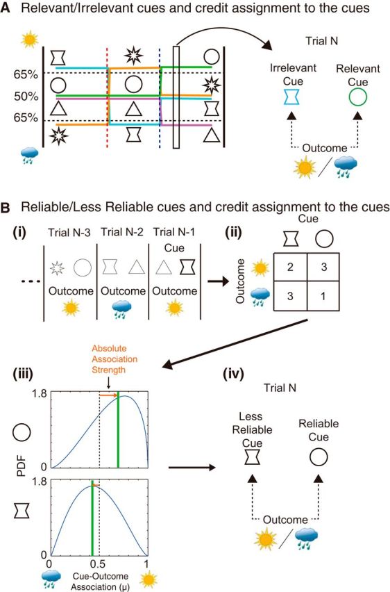
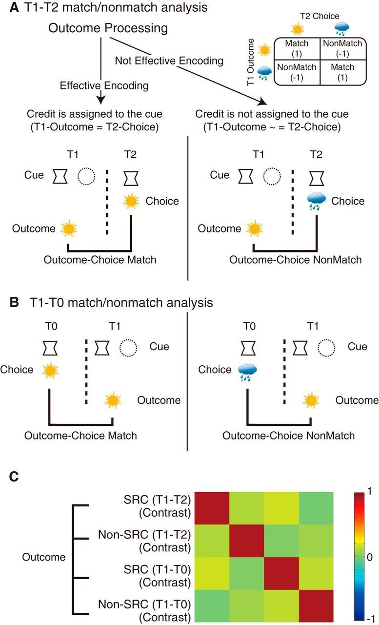
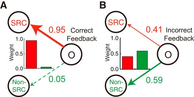
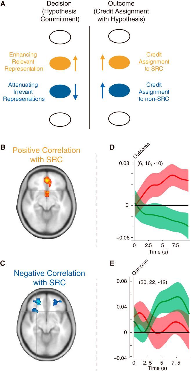
In complex environments, many potential cues can guide a decision or be assigned responsibility for the outcome of the decision. We know little, however, about how humans and animals select relevant information sources that should guide behavior. We show that subjects solve this relevance selection and credit assignment problem by selecting one cue and its association with a particular outcome as the main focus of a hypothesis. To do this, we examined learning while using a task design that allowed us to estimate the focus of each subject's hypotheses on a trial-by-trial basis. When a prediction is confirmed by the outcome, then credit for the outcome is assigned to that cue rather than an alternative. Activity in medial frontal cortex is associated with the assignment of credit to the cue that is the main focus of the hypothesis. However, when the outcome disconfirms a prediction, the focus shifts between cues, and the credit for the outcome is assigned to an alternative cue. This process of reselection for credit assignment to an alternative cue is associated with lateral orbitofrontal cortex.

Significance statement: Learners should infer which features of environments are predictive of significant events, such as rewards. This "credit assignment" problem is particularly challenging when any of several cues might be predictive. We show that human subjects solve the credit assignment problem by implicitly "hypothesizing" which cue is relevant for predicting subsequent outcomes, and then credit is assigned according to this hypothesis. This process is associated with a distinctive pattern of activity in a part of medial frontal cortex. By contrast, when unexpected outcomes occur, hypotheses are redirected toward alternative cues, and this process is associated with activity in lateral orbitofrontal cortex.

Keywords: decision making; learning; medial prefrontal cortex; orbitofrontal cortex.

Figure 1.

Experimental task design and behavioral results. A, Experimental task. Subjects were presented with two geometrical shapes (from a set of four) in the screen center and, separately, two possible weather prediction options at the left and right of the screen. The two cues predict different outcomes as being more likely (percentages indicated above the cues). B, After the presentation of the information cues and the choice options (Cue & Option Display), they chose one weather prediction by pressing a button (Response & Chosen Option Display), and received feedback about the actual weather outcome (Outcome). C, At each phase of the task schedule, two of four cues were predictive of a weather outcome (relevant cues), while the other two cues were not (irrelevant cues). Two types of changes in association between cues and weather outcomes occurred during the task. During reversal switches, the association of the cue with a specific weather outcome was reversed. During Relevance Switches, the predictive cues became nonpredictive and nonpredictive cues became predictive.

Figure 2.

Procedure for estimating subjective cue selection. A, Subjective cue selection (identifying the SRC vs the non-SRC). i, The cue–choice association history reflects each participant's subjective estimate of cue–outcome association. ii, iii, The number of associations between each cue and each choice were, therefore, tallied and discounted with recency-weighted factor of a half-life of six trials (ii) and used to create (iii) β functions (mean value indicated by green lines) summarizing estimates of the subjective strengths of association between each cue and each outcome. iv, These estimates were then compared with the actual choice in the current trial (Trial N). The SRC (shown in red), as opposed to the non-SRC (shown in green), can then be inferred as the cue that was more likely to have guided the participant's choice on the current trial. B, In summary, on each trial, we were able to define the cue that better predicted the subject's current choice as the SRC and the other cue as the non-SRC.

Figure 3.

Procedures of models estimating objective cue selection. A, Predetermined or objective cue relevance (identifying the objectively relevant vs the irrelevant cue). The cue that was objectively of greater relevance for decision making could be determined by the true cue–outcome association history in a given task phase. This corresponds to the cue–outcome association history preprogrammed by the experimenter. In each task phase, two cues were predetermined to be relevant for decision making because of their reliable associations with outcomes (e.g., here, the circle and triangle in the final task phase), while the other two cues were irrelevant for decision making because of their lack of reliable association with outcomes (e.g., here, the hourglass and star cues in the final task phase). B, Cue–outcome reliability in recent history (identifying the recently more reliable vs less reliable cue). i, The designations of the reliable and less reliable cues were based on the cue–outcome associations actually experienced in the recent trial history. ii, iii, The numbers of associations between each cue and each outcome were tallied and discounted with recency-weighted factor of a half-life of six trials (ii) and used to create (iii) a β function, from which the recent predictive reliability of the cues was estimated (inverse of the width of the distribution). iv, The reliability of each of the two cues presented on a given trial was compared to determine which was designated the reliable cue and which was designated the less reliable cue.

Figure 4.

GLM for decision phase analysis. Correlation matrix of regressors in the first fMRI GLM that focused on decision making. The regressors include subjective association strength of the SRC (parametric regressor aligned to decision), the subjective association strength of the non-SRC (parametric regressor aligned to decision), correct/incorrect feedback (1 and −1; contrast regressor aligned to outcome), and RTs (parametric regressor aligned to decision). Magnitudes of correlations are indicated in colors as shown in the color bar (right).

Figure 5.

Procedure of fMRI analysis at outcome. A, For the fMRI analysis, we are interested in the contrast of the brain states that reflect effective encoding of the current outcome and the brain states that do not reflect effective encoding. We assumed that effective encoding of outcome on a given trial T1 (T1 Outcome) in relation to a specific cue led to the subsequent choice of weather predictions (T2 Choice), which was consistent with the previously experienced outcome (left case, effective encoding at T1). The T2 trials were defined as the subsequent trials when the same cue appeared again. If the encoding of the outcome was not effective at T1, the T1 outcome and T2 choice were less likely to be the same (right, not effective encoding at T1). T1 outcome and T2 choice could be either sun or rain. If they were the same (sun–sun or rain–rain), they were treated as match cases. Otherwise, they were treated as nonmatch cases. The contrasts of the two cases were used for the construction of regressors in the fMRI analyses (inset at top right) for each cue. B, T1 outcome and T0 choice regressors were used as control regressors to account for the part of variance that corresponded to the perseverative tendency of choice in response to a specific cue. Here, T0 means a last trial when the same cue appeared. C, Correlation matrix of regressors in the first GLM. The regressors aligned to outcome included the T1–T2 match/nonmatch contrast of the SRC, the T1–T2 match/nonmatch contrast of the non-SRC, the T1–T0 match/nonmatch contrast of the SRC, and the T1–T0 match/nonmatch contrast of the non-SRC. Magnitudes of correlations are indicated in colors as shown in the color bar (right).

Figure 6.

Learning curves after switches. A, Performances are displayed as the percentage of responses to the two-cue compound that were of the optimal type according to the postswitch contingency. Compared with Value Switch (shown in red), the learning speed after Relevance Switch (shown in blue) was much slower. Each bin contains data from 20 trials. B, The same data as in A are replotted with the bin size of 10 trials. The range of the trials is now from 10 trials before switch to 40 trials after switch. Data are presented as mean ± SE across 24 subjects.

Figure 7.

Model comparison. The models of subjective cue selection are shown in black bars. Compared with the basic association model without differential treatment of cues (Basic RL model; Model 1), the model that differentiated SRC and non-SRC at decision stage (Fig. 2; Model 2) explained the subjects' behavior better. The model with differential weighting of the cues at the learning stage (Model 3) explained the subjects' behavior better than the basic model (Model 1). However, this model did not distinguish situations in which the subjects' predictions either matched the weather outcome (correct feedback) or not (incorrect feedback). The model distinguishing the two situations (Model 4) performed still better than the model that did not (Model 3). In fact, Model 4 performed better than any other model (also see Table 1). The models with differential cue weighting based on predetermined cue relevance (Fig. 3A; Predetermined Relevance Weight Model; Models 5–6) are shown in two dark gray bars. The models of recent cue–outcome association history (Fig. 3B; Cue–Outcome Reliability Weight Model; Models 7–9) are shown in three light gray bars. These objective models were not better than Model 1 (also see Table 2).

Figure 8.

Subjective cue selection and learning after switch. A, In the period between 1 and 20 trials immediately after Relevance Switch, the probability of cue selection was higher for the cue that had previously been relevant but was currently irrelevant compared with the cue that was previously irrelevant but became relevant after the Relevance Switch. Data are presented as mean ± SE across 24 subjects. B, The values of the estimated parameters in Model 2 (Table 1) showed that the weight of the SRC was higher (0.82) than that of the non-SRC (0.18). However, if we apply the free parameter only to unambiguous cases when the difference of the association strengths was >0.3 (the dots outside shaded area in C), the weights were 0.99 for SRC and 0.01 for non-SRC. C, Trials were distinguished according to the difference of the association strengths of cues to outcomes. The ambiguous trials were in the shaded area (<0.3), and unambiguous trials were outside the shaded area (>0.3). Axes correspond to association strengths of two cues present in a given trial. D, The probability of selecting the newly relevant (previously irrelevant) cue as SRC was correlated with the probability of optimal choice in the first 1–20 trials after Relevance Switch (r = 0.63, p = 0.0010). E, Probability of selecting the previously relevant (currently irrelevant) cue as SRC was negatively correlated with probability of optimal choice in the first 1–20 trials after Relevance Switch (r = −0.52, p = 0.0087). Each point represents a value from a single subject.

Figure 9.

Learning weights after correct and incorrect feedback. A, In the situation when the subjects' predictions matched the weather outcome (correct feedback), the subjects attributed the outcome almost solely to the cue they used to generate the prediction (SRC in the panel). Almost no learning occurred for the other cue (non-SRC in the panel). The learning weights of cues are displayed in bar graphs: a red bar for the SRC; and a green bar for the non-SRC. B, When the subjects' predictions did not match the weather outcome (incorrect feedback), the subjects attributed the outcome more to the cue they did not use in prediction (non-SRC in the panel). Nevertheless, subjects also attributed part of the cause for the outcome to the cue they did use in prediction (SRC in the panel). Conventions are the same as in A.

Figure 10.

The relationship between decision-related activity and outcome-related activity. A, Neural activity at decision and outcome. The behavioral evidence summarized in Figure 2, A and B, demonstrate that one of the cues present on each trial is selected as the SRC. In this selection process, we reasoned, representation of the SRC is enhanced and the representation of the non-SRC is attenuated. These enhancements and attenuations might take place in different brain regions. In the outcome phase of the task, the brain region with activity correlated with SRC is involved in credit assignment to the SRC. By contrast, the brain region with activity negatively correlated with SRC at the time of decision making should become active in the outcome phase of the trial when a prior hypothesis is disconfirmed, and an alternative hypothesis is considered and credit is assigned to the non-SRC. B, C, Positive and negative correlation with association strength of SRC. The brain regions that, at the time of decision making, showed a positive correlation between activity and the association strength of the SRC were in the MFC. On the other hand, the brain regions with a negative correlation between activity and the association strength of the SRC, at the time of decision making, were in lOFC. This suggests that the MFC and lOFC correspond to the orange and blue mechanisms highlighted on the left-hand side of A above. D, ROI analysis was used to examine the neural activity related to credit assignment to the SRC in MFC. The MFC region that initially showed activity enhancement for the SRC exhibited learning related activity (match/nonmatch contrast), specifically for the SRC (red curve) but not for the non-SRC (green curve). E, ROI analysis of neural activity related to credit assignment to the non-SRC in lOFC. The lOFC area that initially showed activity negatively correlated with the SRC exhibited learning related activity (match/nonmatch contrast) specifically for the non-SRC (green curve) but not for the SRC (red curve).

References

1. Abe H, Lee D. Distributed coding of actual and hypothetical outcomes in the orbital and dorsolateral prefrontal cortex. Neuron. 2011;70:731–741. doi: 10.1016/j.neuron.2011.03.026. - DOI - PMC - PubMed
1. Beckmann CF, Jenkinson M, Smith SM. General multilevel linear modeling for group analysis in FMRI. Neuroimage. 2003;20:1052–1063. doi: 10.1016/S1053-8119(03)00435-X. - DOI - PubMed
1. Beckmann M, Johansen-Berg H, Rushworth MF. Connectivity-based parcellation of human cingulate cortex and its relation to functional specialization. J Neurosci. 2009;29:1175–1190. doi: 10.1523/JNEUROSCI.3328-08.2009. - DOI - PMC - PubMed
1. Behrens TE, Woolrich MW, Walton ME, Rushworth MF. Learning the value of information in an uncertain world. Nat Neurosci. 2007;10:1214–1221. doi: 10.1038/nn1954. - DOI - PubMed
1. Boorman ED, Behrens TE, Woolrich MW, Rushworth MF. How green is the grass on the other side? Frontopolar cortex and the evidence in favor of alternative courses of action. Neuron. 2009;62:733–743. doi: 10.1016/j.neuron.2009.05.014. - DOI - PubMed
Publication types
LinkOut - more resources