Functional Topography of Human Auditory Cortex

Abstract

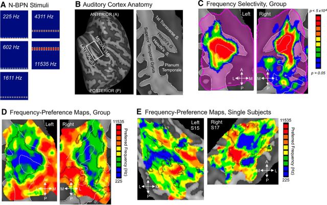
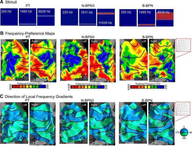
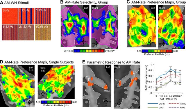
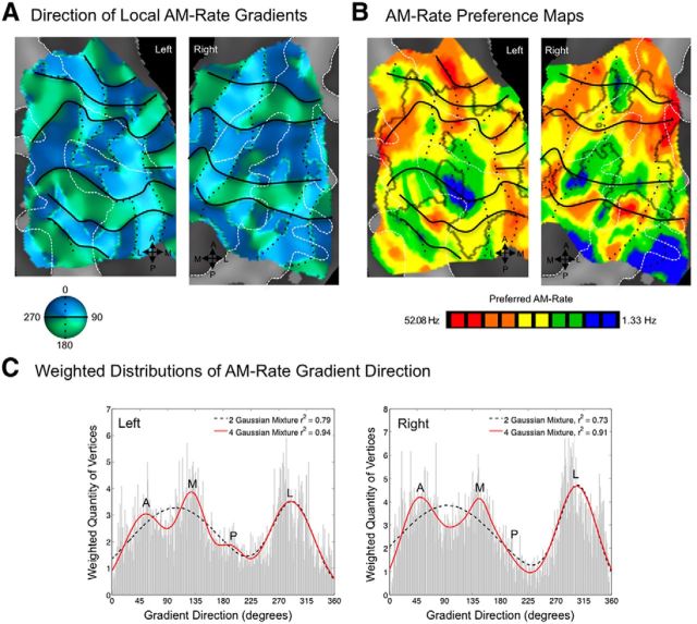
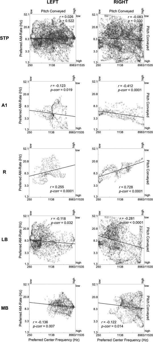
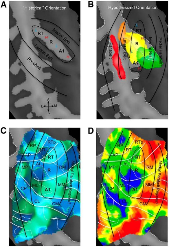
Functional and anatomical studies have clearly demonstrated that auditory cortex is populated by multiple subfields. However, functional characterization of those fields has been largely the domain of animal electrophysiology, limiting the extent to which human and animal research can inform each other. In this study, we used high-resolution functional magnetic resonance imaging to characterize human auditory cortical subfields using a variety of low-level acoustic features in the spectral and temporal domains. Specifically, we show that topographic gradients of frequency preference, or tonotopy, extend along two axes in human auditory cortex, thus reconciling historical accounts of a tonotopic axis oriented medial to lateral along Heschl's gyrus and more recent findings emphasizing tonotopic organization along the anterior-posterior axis. Contradictory findings regarding topographic organization according to temporal modulation rate in acoustic stimuli, or "periodotopy," are also addressed. Although isolated subregions show a preference for high rates of amplitude-modulated white noise (AMWN) in our data, large-scale "periodotopic" organization was not found. Organization by AM rate was correlated with dominant pitch percepts in AMWN in many regions. In short, our data expose early auditory cortex chiefly as a frequency analyzer, and spectral frequency, as imposed by the sensory receptor surface in the cochlea, seems to be the dominant feature governing large-scale topographic organization across human auditory cortex.

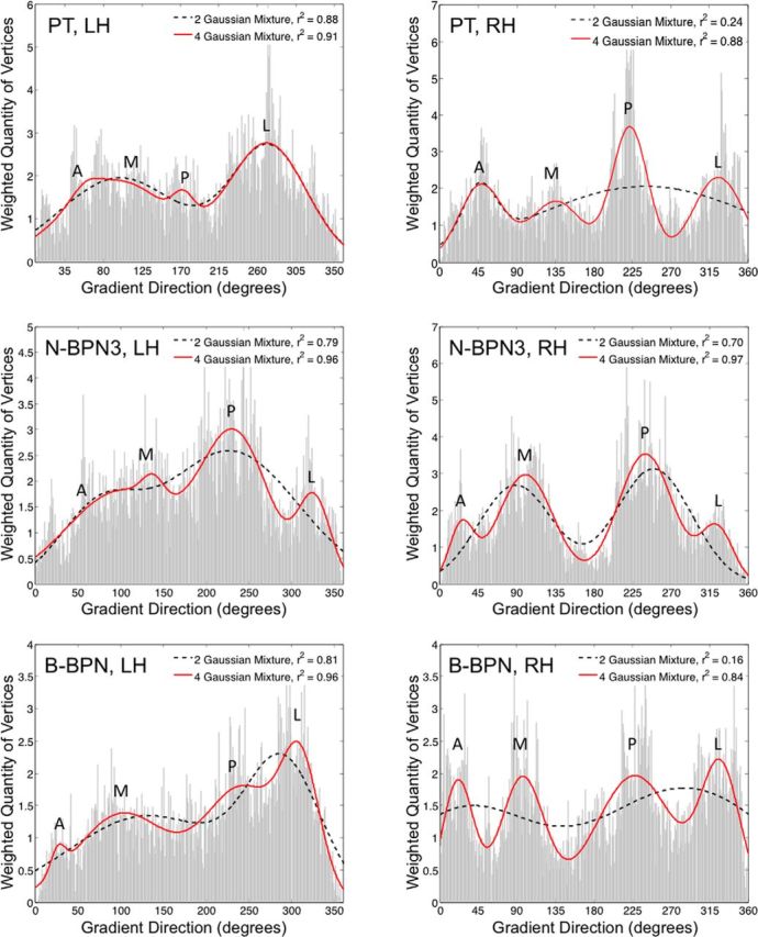
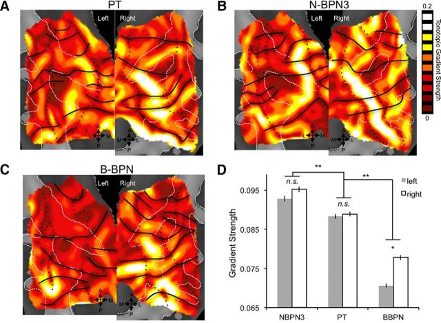
Significance statement: In this study, we examine the nature of topographic organization in human auditory cortex with fMRI. Topographic organization by spectral frequency (tonotopy) extended in two directions: medial to lateral, consistent with early neuroimaging studies, and anterior to posterior, consistent with more recent reports. Large-scale organization by rates of temporal modulation (periodotopy) was correlated with confounding spectral content of amplitude-modulated white-noise stimuli. Together, our results suggest that the organization of human auditory cortex is driven primarily by its response to spectral acoustic features, and large-scale periodotopy spanning across multiple regions is not supported. This fundamental information regarding the functional organization of early auditory cortex will inform our growing understanding of speech perception and the processing of other complex sounds.

Keywords: auditory cortex; fMRI; tonotopy.

Figure 1.

Frequency selectivity in human auditory cortex. A, N-BPN stimuli are displayed in spectrograms; x-axes span 0 to 3 s, and y-axes span 0 to 16 kHz (linear scale). B, The anatomy of the superior temporal cortex is shown using a reconstruction of a group-averaged cortical surface (left), flattened to display all structures in the same plane (right). The borders of major sulci and gyri are marked with white dashed lines. In all subsequent figures, data are presented in this manner, on flattened cortical surfaces with sulci/gyri outlined in white dashed lines. C, Voxels with statistically different BOLD responses to five frequencies of N-BPN are shown, indicating clear frequency selectivity. Such voxels were present throughout the left and right superior temporal plane (key at right; right hemisphere flipped around the AP axis to match the left). D, Group frequency-preference maps or tonotopic maps are shown, whereby color represents the preferred stimulus frequency (i.e., the frequency with the highest BOLD response), as shown in the key at right. Black outlines mark the outline of the clusters from B. E, Single-subject maps of preferred frequency are displayed for two representative subjects (S15, S17). Black outlines mark regions of significant frequency selectivity for each subject as for group maps in D (p < 0.01).

Figure 2.

Measuring tonotopic gradients. A, Stimuli are displayed in spectrograms for PTs, N-BPN (3 frequencies; N-BPN3), and B-BPN; x-axes span 0 to 2.6 s, and y-axes span 0 to 16 Hz (linear scale). B, Group frequency-preference (tonotopic) maps are shown on cortical surfaces; color indicates the center frequency eliciting the greatest BOLD activity. Data for three stimulus types are shown, including PT, N-BPN3, and B-BPN. Note the similarity between N-BPN3 and N-BPN maps in Figure 1D. Isofrequency contours are marked as black (solid and dotted) lines based on frequency reversals determined from gradient maps in C. C, Local frequency gradients are displayed, where color indicates the gradient direction at each point on the tonotopic maps from B, moving from low to high frequencies. Black lines mark gradient reversals between 0/360 and 180° (green to blue, respectively), and black dotted lines mark reversals between 90 and 270° (dark to light colors, respectively). An example of gradient flow is illustrated in a red inset at the right in B and C, and the corresponding points on the rightmost maps are marked. Arrows indicate the direction of tonotopic gradient flow, from low to high frequencies.

Figure 3.

Quantifying tonotopic frequency gradients. For each tonotopic map, the quantity of vertices (i.e., points on the map) exhibiting a given tonotopic gradient direction are displayed. Distributions are given for left- and right-hemisphere maps in left and right columns, respectively, and for PT, N-BPN3, and B-BPN maps in the top, middle, and bottom rows, respectively. Functions containing mixtures of two (black dashed lines) or four (red lines) Gaussians/peaks were fitted to each distribution to assess overall patterns in gradient direction in each tonotopic map. The amount of variance accounted for by these two- and four-Gaussian mixtures is displayed in insets (r² value). Additional goodness-of-fit measures were compatible with r² values; both the AIC and BIC were less for four- than two-Gaussian models, indicating a better fit (two-Gaussian model AIC, −2.84, −3.12, −2.36; four-Gaussian model AIC, −4.44, −3.41, −4.02; two-Gaussian model BIC, −2.78, −3.06, −2.29, four-Gaussian model BIC, −4.31, −3.28, −3.89 for PT, N-BPN3, B-BPN, respectively). The approximate gradient direction is indicated for each peak: A, anterior; M, medial; P, posterior; L, lateral.

Figure 4.

Strength of tonotopic gradients in human auditory cortex. A–C, Strength of frequency organization is displayed for tonotopic gradients in maps for PT (A), N-BPN (B), and B-BPN stimuli (C). Reversals in frequency organization are marked as in Figure 2B. A region of high gradient strength is located near central Heschl's gyrus and sulcus, and may correspond to A1. D, Average gradient strength is plotted for each of the maps in A–C; error bars reflect the SEM across map voxels. Significant differences between stimulus bandwidths are shown by double asterisks. A significant hemisphere by stimulus bandwidth interaction is marked with a single asterisk.

Figure 5.

Selectivity for rates of temporal modulation in white noise. A, AMWN stimuli are displayed in spectrograms; x-axes span 0–2.6 s, and y-axes span 0–16 kHz (linear scale). B, Voxels with statistically different BOLD responses to six temporal rates of AMWN are located on medial (mHG) and lateral HG (lHG), and adjacent superior temporal gyrus. Color marks significant voxels (p < 0.05); a key is given at the right. C, Group maps for preferred modulation rate are shown, where the color of each voxel represents the preferred AM rate (i.e., the rate with the highest BOLD response), as shown in the key on the side. D, Single-subject maps of preferred modulation rate are displayed, with black outlines indicating regions with statistically different BOLD responses to the six AMWN stimuli for each subject. E, Significant parametric relationships between BOLD activity and AM rate are displayed in orange (p_corr < 0.05), with mean activity per AM-rate condition plotted for each of these clusters at right. The asterisk marks a subthreshold cluster on the right mHG (p < 0.005, k = 112 mm³).

Figure 6.

Topographic organization by preferences for temporal modulation rate in auditory cortex. A, Gradient maps for preferred AM rate are shown, where color indicates the gradient direction moving from low to high AM rates. Black lines mark gradient reversals between 0/360 and 180° (green to blue, respectively), and black dotted lines mark reversals between 90 and 270° (dark to light colors, respectively). B, Group maps of AM rate preferences are displayed on cortical surfaces; color indicates the rate eliciting the greatest BOLD activity. Reversals from A are displayed, marking contours sharing similar responses to AM rate in B. C, Distributions are plotted for vertices exhibiting local gradient directions 0–360°, weighted by the strength of the gradient at each vertex. Functions containing mixtures of two (black dashed lines) or four (red lines) Gaussians were fitted to the shape of these distributions to assess overall patterns in gradient direction. A goodness of fit (r² value) for two- and four-Gaussian mixtures is displayed in the upper right corner of each box. Additional goodness-of-fit measures were compatible with r² values; the AIC and BIC were less for four- than two-Gaussian models, indicating a better fit (AIC, −1.92 and −3.08 for two- and four-Gaussian models; BIC, −1.86 and −2.95 for two and four-Gaussian models, respectively). A, Anterior; M, medial; P, posterior; L, lateral.

Figure 7.

Spatial correspondence between AM-rate maps and tonotopic maps for all of auditory cortex (top row) and selected regions/areas of auditory cortex (bottom rows). Scatter plots are shown, where each data point represents each voxel's preferred rate of AMWN (left y-axis) and preferred spectral center frequency (bottom x-axis). Dominant pitch conveyed is also displayed for AMWN (right y-axis) and center frequency (top x-axis). Negative correlations suggest that AM-rate preference might be explained by spectral/pitch information conveyed by AMWN stimuli. Data for preferred center frequency were taken from group tonotopic maps including all stimulus bandwidths (i.e., PT, N-BPN, and B-BPN). Black lines mark the best linear fit to each scatter plot (Pearson's r). Auditory cortical fields analyzed include the entire STP, putative core subfields A1 and R, the lateral belt (LB), and the medial belt (MB).

Figure 8.

Hypothesized positions of auditory cortical regions coincide with probabilistic maps of koniocortical areas in humans. A, Previous neuroimaging research placed the orientation of core auditory fields along HG, with high frequencies represented medially (red “H”) and low frequencies represented laterally (blue “L”). B, Our current data confirm an orientation of core regions oblique to HG, with high and low frequencies alternating from posterior to anterior. In this scheme, our functional definition of core regions overlaps with the koniocortical/primary region Te1.0, as defined from underlying cytoarchitecture (Morosan et al. 2001; Rademacher et al., 2002), which is shown in yellow according to the Wake Forest University PickAtlas (Maldjian et al., 2003). Medial, nonprimary region Te1.1 is shown in green, the lateral region Te1.2 in orange, and Te3.0 in red. C, A map of frequency-gradient direction is shown, derived from a map of frequency preference independent of stimulus bandwidth (i.e., including responses to PT, N-BPN, and B-BPN together). White lines indicate the position of gradient reversals as in Figures 2 and 6. The hypothesized locations of the putative core, belt, and parabelt regions are marked by solid black lines, along with hypothesized subregions homologous to those identified in nonhuman primates. D, A group tonotopic map is displayed, which matches gradient map displayed in C. Data from all stimulus frequencies and bandwidths were used to create this map. Reversals that appear to delineate subregions in C remain in D. All panels display a group-average cortical surface (right hemisphere), and white dashed lines mark major sulci and gyri. Auditory subfield names are taken from the nonhuman primate literature for convenience and follow these abbreviations: R, rostral; C, caudal; M, medial; A, anterior; L, lateral belt; P, parabelt; T, temporal; p, pole. Note that “M” refers to “medial belt” when occurring as the second letter of a two-letter abbreviation (e.g., CM, caudomedial belt).

References

1. Alho K, Grimm S, Mateo-León S, Costa-Faidella J, Escera C. Early processing of pitch in the human auditory system. Eur J Neurosci. 2012;36:2972–2978. doi: 10.1111/j.1460-9568.2012.08219.x. - DOI - PubMed
1. Barton B, Venezia JH, Saberi K, Hickok G, Brewer AA. Orthogonal acoustic dimensions define auditory field maps in human cortex. Proc Natl Acad Sci U S A. 2012;109:20738–20743. doi: 10.1073/pnas.1213381109. - DOI - PMC - PubMed
1. Baumann S, Griffiths TD, Sun L, Petkov CI, Thiele A, Rees A. Orthogonal representation of sound dimensions in the primate midbrain. Nat Neurosci. 2011;14:423–425. doi: 10.1038/nn.2771. - DOI - PMC - PubMed
1. Baumann S, Petkov CI, Griffiths TD. A unified framework for the organization of the primate auditory cortex. Front Syst Neurosci. 2013;7:11. doi: 10.3389/fnsys.2013.00011. - DOI - PMC - PubMed
1. Baumann S, Joly O, Rees A, Petkov CI, Sun L, Thiele A, Griffiths TD. The topography of frequency and time representation in primate auditory cortices. Elife. 2015;4:e03256. doi: 10.7554/eLife.03256. - DOI - PMC - PubMed
Publication types