. 2016 Mar;115(3):1644-53.
doi: 10.1152/jn.00842.2015. Epub 2016 Jan 28.

Recording and labeling at a site along the cochlea shows alignment of medial olivocochlear and auditory nerve tonotopic mappings

Affiliations

Recording and labeling at a site along the cochlea shows alignment of medial olivocochlear and auditory nerve tonotopic mappings

M Christian Brown. J Neurophysiol. 2016 Mar.

Abstract

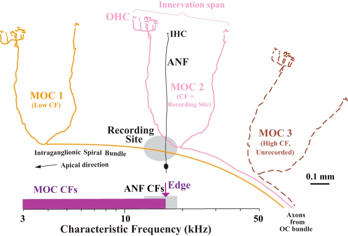
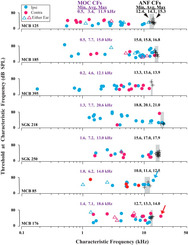
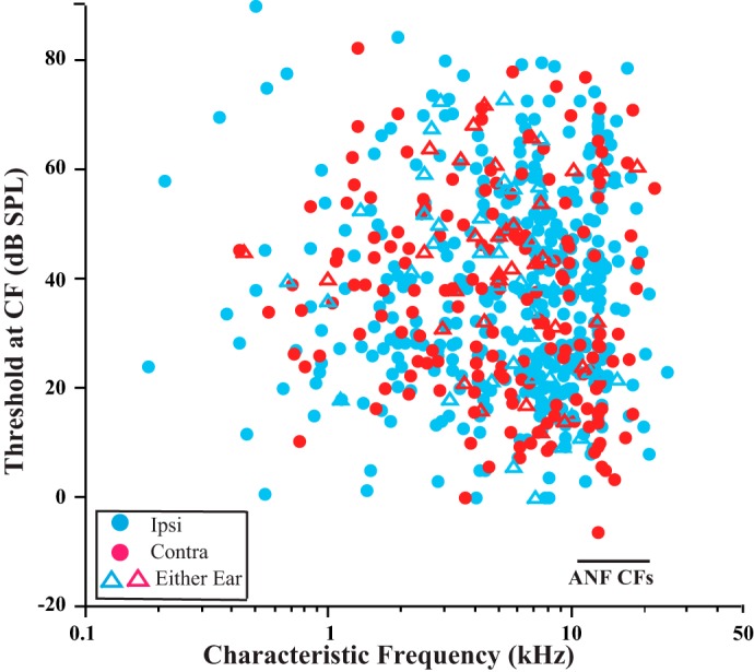
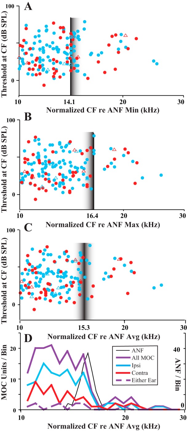
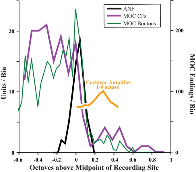
Medial olivocochlear (MOC) neurons provide an efferent innervation to outer hair cells (OHCs) of the cochlea, but their tonotopic mapping is incompletely known. In the present study of anesthetized guinea pigs, the MOC mapping was investigated using in vivo, extracellular recording, and labeling at a site along the cochlear course of the axons. The MOC axons enter the cochlea at its base and spiral apically, successively turning out to innervate OHCs according to their characteristic frequencies (CFs). Recordings made at a site in the cochlear basal turn yielded a distribution of MOC CFs with an upper limit, or "edge," due to usually absent higher-CF axons that presumably innervate more basal locations. The CFs at the edge, normalized across preparations, were equal to the CFs of the auditory nerve fibers (ANFs) at the recording sites (near 16 kHz). Corresponding anatomical data from extracellular injections showed spiraling MOC axons giving rise to an edge of labeling at the position of a narrow band of labeled ANFs. Overall, the edges of the MOC CFs and labeling, with their correspondences to ANFs, suggest similar tonotopic mappings of these efferent and afferent fibers, at least in the cochlear basal turn. They also suggest that MOC axons miss much of the position of the more basally located cochlear amplifier appropriate for their CF; instead, the MOC innervation may be optimized for protection from damage by acoustic overstimulation.

Keywords: afferent; characteristic frequency; cochlear amplifier; efferent; outer hair cell.


Figures

Fig. 1.
Fig. 1.
Schematic of the cochlear innervation by medial olivocochlear (MOC) axons (colors) and auditory nerve fibers (ANFs; black), shown in relation to a recording site (gray oval) in the spiral ganglion. Three MOC axons are shown entering the cochlea from the OC bundle at right. The axons run apically in the intraganglionic spiral bundle and terminate onto outer hair cells (OHC) at different positions along the cochlea. For simplicity, the drawings are duplicates of an axon from a single-unit labeling study (Brown 2014). Axons MOC 1 and MOC 2 can be sampled because they take a spiral course through the recording site, but axon MOC 3 cannot be sampled because before it reaches the site it turns out to terminate basally at a location appropriate for its high characteristic frequency (CF). The ANF can be sampled because it takes a radial course through the recording site from a single inner hair cell (IHC) to its cell body in the spiral ganglion. The scale at bottom shows the expected CF distributions: for MOC units (purple), a broad pattern with an upper limit, or “edge,” and for ANFs (gray), a narrow pattern. The CF scale is exaggerated and would span much of the basal turn, rather than just the small portion schematized here. The type of ANF shown is termed “type I”; not shown are unmyelinated ANFs, termed “type II,” which provide contacts on OHCs. Unmyelinated lateral OC fibers that innervate the IHCs also are not shown.
Fig. 2.
Fig. 2.
Data illustrating that MOC CFs (colored symbols) are distributed in a broad pattern up to an upper limit, or edge, at the CF of ANFs (black symbols). Data are from 7 individual guinea pigs; CF minimums, averages, and maximums (Min, Avg, Max) are given for each animal. For ANFs, the narrow range of CFs (gray shading) differs from case to case because of differences in placement of the recording site in each cochlea. The guinea pigs in the 2 lowermost plots had exceptional MOC units with CFs above those of ANFs (colored arrows). Ipsi units are driven by sound in the ipsilateral ear, contra units by sound in the contralateral ear, and either-ear units by sound in either ear.
Fig. 3.
Fig. 3.
Pooled distribution of CFs of all MOC units. Data are 639 MOC units from 133 guinea pigs. Horizontal bar indicates the overall range for CFs of ANFs (9.64 to 22.6 kHz).
Fig. 4.
Fig. 4.
Normalized MOC data to allow for comparisons of the CF edge of all units across preparations. Normalization was done for each particular guinea pig according to 3 measures of the CFs of ANFs in that guinea pig. A: CFs multiplied by 14.1/(ANF CFmin), where ANF CFmin is the minimum CF of the ANF from the preparation in which the MOC unit was recorded. B: CFs multiplied by 16.4/(ANF CFmax), where ANF CFmax is the maximum CF of the ANF from the preparation. C: CFs multiplied by 15.3/(ANF CFavg), where ANF CFavg is the average CF of the ANF from the preparation. The multipliers (14.1, 16.4, or 15.3) were chosen because they are the average minimum CF, average maximum CF, and average CF (in kHz) across the preparations of the study. Vertical lines indicate the points of alignment based on ANF measures, and fuzzy borders are meant to indicate nonalignment of ANF CFs there. D: binned data using average normalized MOC CFs (same x-axis as C) and ANF data consisting of 145 units from the 12 guinea pigs in which 8 or more ANFs were recorded.
Fig. 5.
Fig. 5.
Proportions of units for each response type. A: all MOC units. B and C: MOC normalized CFs over the range 10–16.4 kHz (B) and for the range above16.4 kHz (C). For normalization, the maximum CF for ANFs was used so that all points in C are MOC units with CFs greater than that of any ANF in that preparation. Numbers of units are indicated for each histogram. A z-test showed no significant difference in proportion of ipsi units in these 2 regions (z = 0.3572, P = 0.71884).
Fig. 6.
Fig. 6.
Patterns of MOC labeling resulting from extracellular injections of neural tracer. Micrograph of the injection site in 1 case (A) and reconstructions of 2 other cases (B and C). In B and C, the dots and fibers represent all labeled MOC endings and tunnel-crossing branches within a half-turn from the injection site. In B, a case with many labeled fibers, the MOC labeling is dense adjacent and apical to the injection site, but it diminishes adjacent to the injection site to become sparse basally (gray arrows). Labeling extends along the organ of Corti for 1,429 μm from the basalmost edge of the labeled peripheral ANFs (gray shaded band). In C, a case with few labeled fibers, the basal labeling consists of only 1 cluster of MOC endings (gray arrow) located 731 μm basal to the ANFs. Ovals indicate labeled cell bodies of the spiral ganglion that give rise to the ANFs. IGSB, intraganglionic spiral bundle.
Fig. 7.
Fig. 7.
Data illustrating that MOC labeling is distributed in a broad pattern approaching a basal limit, or edge, where it drops off at the position of the labeling of ANFs (gray shading). Each graph shows the labeling in an individual cochlea. Points represent the number of MOC endings in 100-μm bins; bins with no endings are not plotted. Arrows indicate MOC labeling more basal than the ANF labeling. Survival times were the longest of the present data set to ensure the most apical labeling and are (from top to bottom) 23.5, 22.5, 13.25, 24, 24, and 12 h. Case 94R was illustrated in Fig. 6B.
Fig. 8.
Fig. 8.
Comparison of MOC labeled endings (A) and staining for acetylcholinesterase (AChE; B). Labeling in A is the same as cases shown in Fig. 7, aligned on the basis of the middle of the ANF labeling. Inset shows an expanded view of endings tabulated separately for the OHC rows. AChE staining used a qualitative scale ranging from 0 (no staining) to 5 (darkest staining) because staining was too dense to resolve individual endings. Results for 1 cochlea are shown in B; the other 3 AChE-stained cochleas had similar patterns.
Fig. 9.
Fig. 9.
Comparison of distributions CFs and MOC endings as plotted on an octave scale. CFs are binned and normalized as in Fig. 4D, and y-axis at left indicates MOC units/bin, or (ANF units/bin)/2 (half the scale used in Fig. 4D). Boutons are binned and aligned as in Fig. 8A, and the CF correlate of their position was computed using the cochlear frequency mapping (Brown 2014). The extent of the cochlear amplifier (yellow curve) is indicated by displacing ANF distribution by 650 μm (one-quarter octave).

References

    1. Adams JC. Technical considerations on the use of horseradish peroxidase as a neuronal marker. Neuroscience 2: 141–145, 1977. - PubMed
    1. Ashmore J, Avan P, Brownell WE, Dallos P, Dierkes K, Fettiplace R, Grosh K, Hackney CM, Hudspeth AJ, Jülicher F, Lindner B, Martin P, Meaud J, Petit C, Santos-Sacchi J, Canlon B. The remarkable cochlear amplifier. Hear Res 266: 1–17, 2010. - PMC - PubMed
    1. Brown MC. Morphology and response properties of single olivocochlear fibers in the guinea pig. Hear Res 40: 93–110, 1989. - PubMed
    1. Brown MC. Morphology of labeled afferent fibers in the guinea pig cochlea. J Comp Neurol 260: 591–604, 1987a. - PubMed
    1. Brown MC. Morphology of labeled efferent fibers in the guinea pig cochlea. J Comp Neurol 260: 605–618, 1987b. - PubMed

Publication types

LinkOut - more resources