Two distinct types of remapping in primate cortical area V4

Abstract

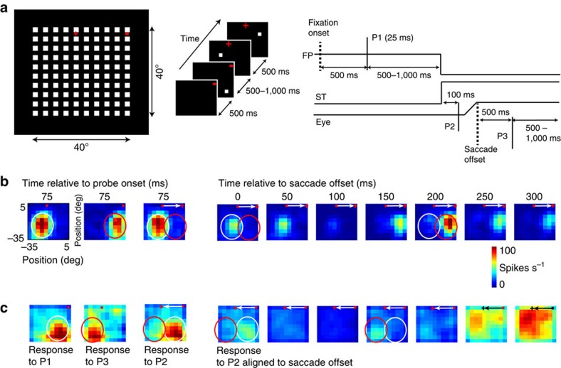
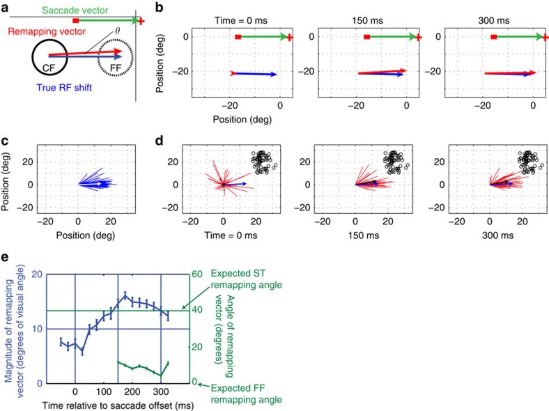
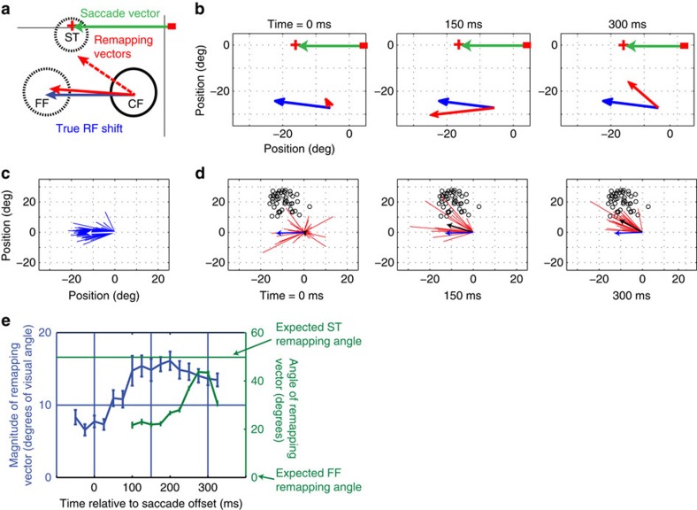
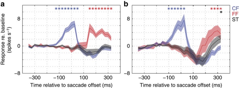
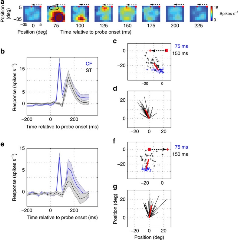
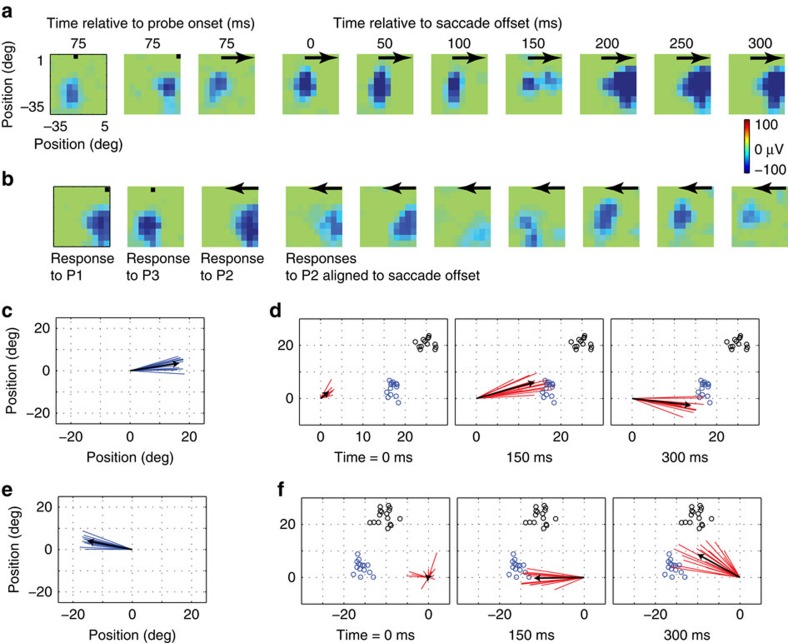
Visual neurons typically receive information from a limited portion of the retina, and such receptive fields are a key organizing principle for much of visual cortex. At the same time, there is strong evidence that receptive fields transiently shift around the time of saccades. The nature of the shift is controversial: Previous studies have found shifts consistent with a role for perceptual constancy; other studies suggest a role in the allocation of spatial attention. Here we present evidence that both the previously documented functions exist in individual neurons in primate cortical area V4. Remapping associated with perceptual constancy occurs for saccades in all directions, while attentional shifts mainly occur for neurons with receptive fields in the same hemifield as the saccade end point. The latter are relatively sluggish and can be observed even during saccade planning. Overall these results suggest a complex interplay of visual and extraretinal influences during the execution of saccades.

Figure 1. Illustration of experimental paradigm and example neurons.

(a) (left) All possible visual probe locations (10 × 10 probe grid) spanning 40° of visual space (figure not drawn to scale for clarity). Fixation point (red dot) and saccade target (red ‘+') indicate the leftward direction of the horizontal, visually guided saccade in this example. (middle) Sequence of visual stimuli on an example trial, including the fixation targets and the appearance of the three probes at random locations. (right) Time course of a single trial. (b) Receptive field of an example neuron for probes flashed during fixation (left two panels; fixation points indicated by red dot) and those flashed immediately before an ‘away saccade' (defined as a saccade directed horizontally away from the hemifield containing the receptive field) indicated by white arrows (third panel: responses aligned to probe onset; and fourth panel and onwards: responses aligned to saccade offset). (c) Receptive field of another example neuron for a ‘towards saccade' (defined as a saccade directed horizontally towards the hemifield contacting the receptive field) (same scheme as in b). FP, fixation point; ST, saccade target.

Figure 2. Quantification of receptive field remapping for away saccades.

(a) A cartoon of the CF (solid black) and the FF (dotted black) of a hypothetical neuron for an away saccade (green arrow). The true receptive field shift is a vector connecting the centres of the CF and FF (blue arrow). Similarly, the actual remapping vector connects the centre of the CF and the centre of the perisaccadic receptive field (red arrow). The magnitude of this vector and its angle of rotation (indicated by θ) relative to the true receptive field shift vector (blue arrow) are used to quantify receptive field remapping. (b) True RF shift vector (obtained by joining RF centres 75 ms after P1 and P3 onset, respectively) and remapping vector of the example neuron from Fig. 1b at different times relative to the saccade offset. (c) True RF shift vectors of the population of 86 neurons. The white arrow indicates the average vector. (d) Remapping vectors of the population of cells at different times relative to saccade offset. The black arrows indicate the average vectors. The blue arrow shows the average true RF shift (same as white arrow in (c)). Since all the RFs are centred at the origin, the saccade target positions vary (indicated by small black circles). (e) Time course of the average magnitude (blue; error bars represent s.e.m. across the population of neurons) and mean direction (green; error bars represent circular s.d.) of the remapping vectors relative to the saccade offset. Vertical lines indicate analysis time points at 150 and 300 ms post saccade, as well as saccade offset at 0 ms. CF, current field; FF, future field.

Figure 3. Quantification of receptive field remapping for towards saccades.

(a) Receptive field geometry, as in Fig. 2a. (b) True RF shift vector (obtained by joining RF centres, 75 ms after P1 and P3 onset, respectively) and remapping vector of the example neuron from Fig. 1c at different times relative to the saccade offset. (c) True RF shift vectors of the population of 54 neurons. The white arrow indicates the average vector. (d) Remapping vectors of the population of cells at different times relative to saccade offset. The black arrows indicate the average vectors. The blue arrow shows the average true RF shift (same as white arrow in (c)). Since all the RFs are centred at the origin, saccade target positions vary (indicated by small black circles). (e) Time course of average magnitude (blue; error bars represent s.e.m. across the population of neurons) and mean direction (green; error bars represent circular s.d.) of the remapping vectors relative to the saccade offset.

Figure 4. Temporal dynamics of different types of remapping in V4.

(a) Average responses to P2 probes flashed at the CF (blue), FF (red) and saccade target location (black) for away saccades (n=83). Baseline responses before the probe onset were subtracted from the response curves. (b) Responses to P2 probes flashed at the CF (blue), FF (red) and saccade target location (black) for towards saccades (n=54). Stars indicate responses that were significantly above baseline (one sample t-test, P<0.05) and shades represent s.e.m. across the respective population of neurons.

Figure 5. Receptive field remapping during fixation.

(a) Time course of the receptive field of an example neuron during fixation. The fixation point is indicated by the red dot, and the saccade target is indicated by the red ‘+, which will appear 500–1,000 ms after P1 probe onset. Dotted arrow indicates an impending saccade after the target appearance. (b) Average temporal dynamics (n=35 neurons) of responses to probes flashed at the CF (blue) (indicated by blue circle in the second panel of Fig. 5a) and those at the saccade target (black) (indicated by black circle in the second panel of Fig. 5a) during fixation before towards saccades. (c) RF centres at visual latency of 75 ms (blue ‘+') and those at 150 ms (black ‘+') after probe onset during fixation at the red dot. The red line indicates the vector connecting the average RF locations at the two time points after probe onset. (d) The black lines represent the vectors connecting the RFs at 75 ms and RFs at 150 ms after probe onset. RFs at 75 ms are aligned for quantifying the average direction of RF shift. (e) Average temporal dynamics (n=31 neurons) of responses to probes flashed at the CF (blue) and those at saccade target (black) during fixation before away saccades. (f) RF centres at visual latency of 75 ms (blue ‘+') and those at 150 ms (black ‘+') after probe onset during fixation at the indicated red dot. (g) Same as d. Shades represent s.e.m. across the respective population of neurons.

Figure 6. Remapping of LFP receptive fields.

(a) LFP receptive field of an example electrode for probes flashed during fixation (left two panels; fixation points indicated by black dot) and those flashed immediately before an away saccade, indicated by black arrows (third panel: responses aligned to probe onset; fourth panel and onwards: responses aligned to saccade offset). (b) LFP receptive field of an example electrode for towards saccades. (c) True LFP RF shift vectors of the population of 14 electrode sites with eccentricity >20°. (d) Remapping vectors of the same population at different times relative to saccade offset. The black arrows indicate average vectors. Since all the RFs are centred at the origin, saccade target positions vary (indicated by small black circles). Each vector's expected FF location (based on P3 RF) is indicated by small blue circle. (e) and (f) show the results from the same analysis as c and d for towards saccade. LFP, local field potential.

References

1. Hubel D. H. & Wiesel T. N. Ferrier lecture. Functional architecture of macaque monkey visual cortex. Proc. R. Soc. Lond. B. Biol. Sci. 198, 1–59 (1977). - PubMed
1. Huberman A. D. et al. Architecture and activity-mediated refinement of axonal projections from a mosaic of genetically identified retinal ganglion cells. Neuron 59, 425–438 (2008). - PMC - PubMed
1. Duhamel J. R., Colby C. L. & Goldberg M. E. The updating of the representation of visual space in parietal cortex by intended eye movements. Science 255, 90–92 (1992). - PubMed
1. Walker M. F., Fitzgibbon E. J. & Goldberg M. E. Neurons in the monkey superior colliculus predict the visual result of impending saccadic eye movements. J. Neurophysiol. 73, 1988–2003 (1995). - PubMed
1. Umeno M. M. & Goldberg M. E. Spatial processing in the monkey frontal eye field. I. Predictive visual responses. J. Neurophysiol. 78, 1373–1383 (1997). - PubMed
Publication types
LinkOut - more resources