Primary visual cortex shows laminar-specific and balanced circuit organization of excitatory and inhibitory synaptic connectivity

Abstract

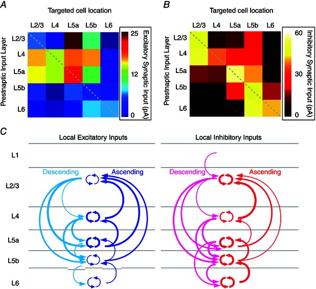
Key points: Using functional mapping assays, we conducted a quantitative assessment of both excitatory and inhibitory synaptic laminar connections to excitatory neurons in layers 2/3-6 of the mouse visual cortex (V1). Laminar-specific synaptic wiring diagrams of excitatory neurons were constructed on the basis of circuit mapping. The present study reveals that that excitatory and inhibitory synaptic connectivity is spatially balanced across excitatory neuronal networks in V1.

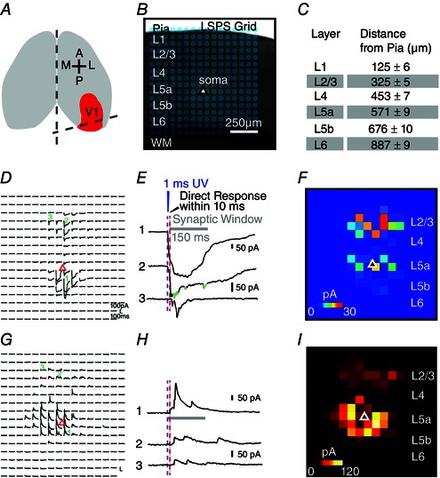
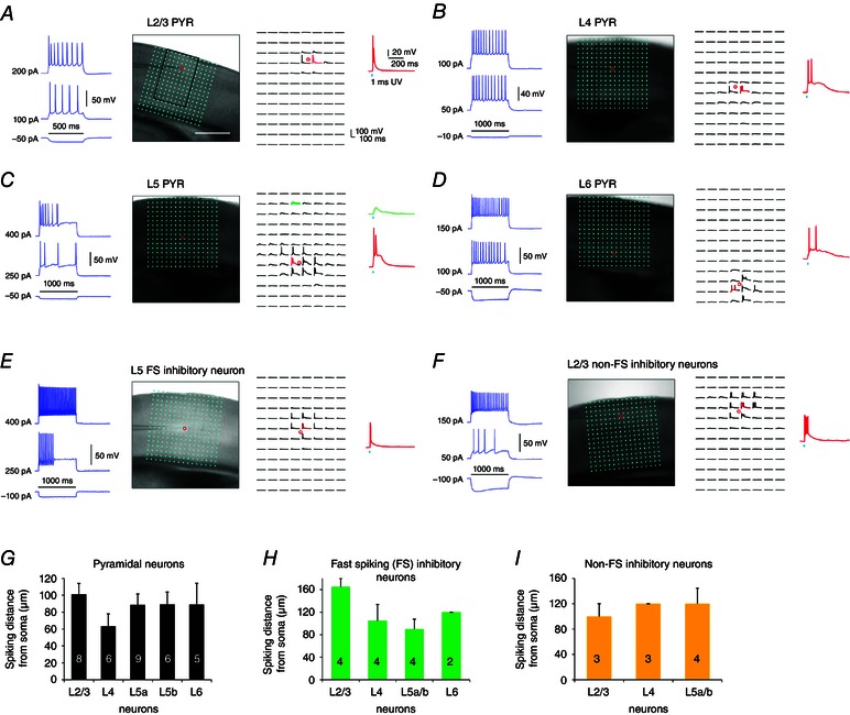
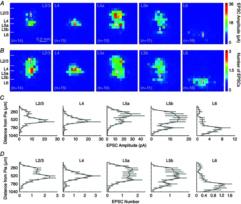
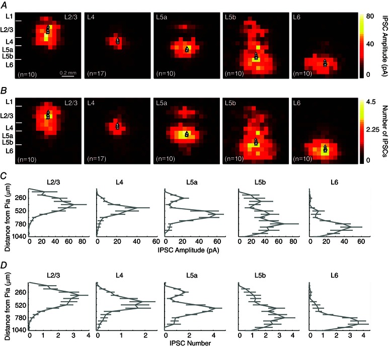
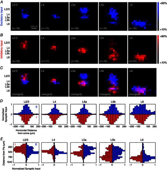
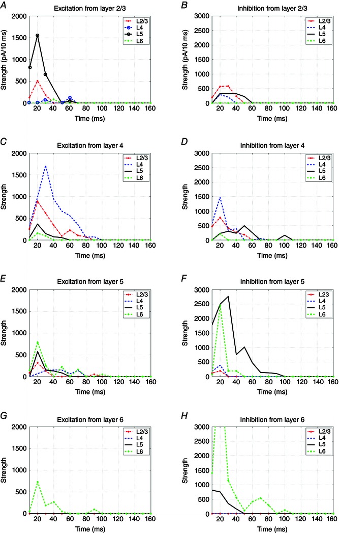
Abstract: In the mammalian neocortex, excitatory neurons provide excitation in both columnar and laminar dimensions, which is modulated further by inhibitory neurons. However, our understanding of intracortical excitatory and inhibitory synaptic inputs in relation to principal excitatory neurons remains incomplete, and it is unclear how local excitatory and inhibitory synaptic connections to excitatory neurons are spatially organized on a layer-by-layer basis. In the present study, we combined whole cell recordings with laser scanning photostimulation via glutamate uncaging to map excitatory and inhibitory synaptic inputs to single excitatory neurons throughout cortical layers 2/3-6 in the mouse primary visual cortex (V1). We find that synaptic input sources of excitatory neurons span the radial columns of laminar microcircuits, and excitatory neurons in different V1 laminae exhibit distinct patterns of layer-specific organization of excitatory inputs. Remarkably, the spatial extent of inhibitory inputs of excitatory neurons for a given layer closely mirrors that of their excitatory input sources, indicating that excitatory and inhibitory synaptic connectivity is spatially balanced across excitatory neuronal networks. Strong interlaminar inhibitory inputs are found, particularly for excitatory neurons in layers 2/3 and 5. This differs from earlier studies reporting that inhibitory cortical connections to excitatory neurons are generally localized within the same cortical layer. On the basis of the functional mapping assays, we conducted a quantitative assessment of both excitatory and inhibitory synaptic laminar connections to excitatory cells at single cell resolution, establishing precise layer-by-layer synaptic wiring diagrams of excitatory neurons in the visual cortex.

Figure 1. V1 slice preparation and LSPS circuit mapping

A, schematic V1 slice preparation: slices are made from mouse primary visual cortex, cut at a 75^o oblique angle relative to midline to preserve intracortical laminar connections. B, illustration of LSPS mapping of local cortical circuit input to single recorded cells. Excitatory neurons are recorded from binocular V1 region in whole cell mode, and the slice image is superimposed with a 16 × 16 LSPS mapping grid (blue dots, 65 μm² spacing) centred around the cell soma (triangle) and is aligned to the pial surface. Laminar boundaries are determined by cytoarchitectonic landmarks in bright‐field slice images, validated by the boundaries determined by post hoc DAPI staining. C, average depth of laminar boundaries measured from the pial surface to the bottom edge of each layer (n = 15 slices). D, representative LSPS excitatory input map from voltage clamping an L5a pyramidal neuron at −70 mV in response to spatially restricted glutamate uncaging in the mapping grid (B). Each trace is plotted at the LSPS location shown in (B). E, detailed view of evoked EPSCs measured from the L5a pyramidal neuron at three respective locations numbered in (D). Trace 1 demonstrates a large ‘direct response’ resulting from uncaging at the perisomatic region. Trace 2 provides an example of a relatively small direct response in L2/3 from uncaging at the apical dendrite coupled with overriding synaptic inputs (shown in green). Trace 3 illustrates synaptic inputs (EPSCs) measured from a L2/3 location. Note the difference of amplitudes and latencies of direct and synaptic input responses, thus allowing for functional characterization. Empirically, responses within the 10 ms window from laser onset are considered direct, and exhibit a distinct shape (shorter rise time) and occurred immediately after glutamate uncaging (shorter latency). Synaptic events (i.e. EPSCs) are measured with the analysis window of >10–160 ms after photostimulation (grey bar). For details, see Methods. F, colour‐coded EPSC input map showing the overall spatial distribution and strength of excitatory inputs to the recorded L5a pyramidal cell. The map is constructed from the responses shown in (D); input responses per location are quantified in terms of average integrated EPSC strength within the analysis window, and colour coded according to the amplitude. G, representative LSPS inhibitory input map from voltage clamping an L5a pyramidal neuron at 5 mV in response to LSPS in the mapping grid similar to (D). H, examples of evoked IPSCs measured in an L5a pyramidal neuron at three respective locations numbered in (G). Trace 1 demonstrates large IPSCs measured near the cell soma. Traces 2 and 3 provide examples of interlaminar inhibition from L2/3. Consistent with excitatory inputs, IPSCs were measured with the analysis window of >10–150 ms after photostimulation (grey bar). I, colour‐coded IPSC input map showing the overall spatial distribution and strength of inhibitory inputs made to the L5a pyramidal cell.

Figure 2. Spatial resolution of photostimulation

A–F, examples of photostimulation‐evoked excitability profiles of pyramidal and inhibitory interneurons in different visual cortical layers. A, current injection responses of an example L2/3 pyramidal neuron are shown on the left; the image of V1 slice where the cell was recorded in layer 2/3 is superimposed with photostimulation sites (*, cyan dots, 65 μm² spacing) (middle) and the photostimulation responses of the recorded neuron are plotted at the beginning of stimulation onset (right). The individual responses are plotted relative to their spatial locations in the mapping array shown in the middle. The small red circle indicates the somatic location of the recorded neuron. One response trace with photostimulation‐evoked APs is indicated in red, and shown separately by the side. Laser flashes (1 ms, 15 mW) were applied for photostimulation mapping. The scale in (A) is 500 μm. B–F, similarly formatted as in (A), with example L4, L5 and L6 pyramidal neurons, and L5 fast spiking inhibitory neurons and L2/3 non‐fast spiking inhibitory neurons, respectively. C, two response traces with photostimulation‐evoked subthreshold depolarization (green, photostimulation at the apical dendrite) and suprathreshold APs (red, perisomatic region) are shown separately. G–I, spatial resolution of LSPS evoked excitability of pyramidal neurons, fast‐spiking and non‐fast spiking inhibitory neurons was determined by measuring the LSPS evoked spike distance relative to soma location. Note that the spiking distance is measured as the ‘vertical’ distance (perpendicular to cortical layers) above and below the cell body. The numbers of recorded neurons are shown at the bar graphs. Data are presented as the mean ± SE.

Figure 3. Morphological profiles of V1 excitatory neurons

Neurons recorded for laminar synaptic input analyses were morphologically examined via biocytin staining. DAPI counterstain was used to establish layer identity. A, representative upper L2/3 pyramidal neuron with truncated apical dendrites. B, excitatory neurons in deeper L2/3 exhibiting longer apical dendrites projecting toward the pial surface. C, almost all L4 excitatory cells recorded confirmed pyramidal cells with apical dendrites projecting toward the pial surface. D–E, L5a and L5b excitatory cells exhibiting typical tall pyramidal cell morphology. F, long L6 pyramidal cell with apical dendrites projecting into L5 and L4. G, example of a L6 pyramidal neuron with short apical dendrites terminating in L5.

Figure 4. Local excitatory inputs to V1 pyramidal neurons

A, group averaged excitatory input maps for excitatory pyramidal cells for each cortical lamina (L2/3, L4, L5a, L5b and L6). Each colour coded pixel represents the average evoked EPSC amplitude across the LSPS mapping grid; white triangles represent the cell body locations of recorded pyramidal neurons. The left most map charts laminar V1 boundaries relative to the 16 × 16 mapping grid based on post hoc DAPI counterstaining. B, numbers of EPSCs per LSPS location are plotted from the averaged maps presented in (A). For normalization, colour‐coded laminar excitatory input maps are scaled to the highest input value across groups. C, EPSC amplitudes are quantified across the radial vector corresponding to the columnar position of recorded cells across layers. D, laminar profiles of EPSC numbers are quantified across the radial vector corresponding to the columnar position of recorded cells throughout the cortical depth, similar to (C). Data are presented as the mean ± SE. For the L2/3 pyramidal cells examined, the average numbers of evoked EPSCs per photostimulation are 1.1 ± 0.3, 1.8 ± 0.4, 1.5 ± 0.5, 0.5 ± 0.3 and 0.2 ± 0.1 for L2/3, L4, L5a, L5b and L6, respectively. The average numbers of evoked EPSCs per photostimulation for L4 pyramidal neurons are 0.5 ± 0.2, 2.2 ± 0.7 and 1.3 ± 0.5 in L2/3, L4 and L5a, respectively. The average numbers of evoked EPSCs per photostimulation for L5 pyramidal neurons are 1.4 ± 0.2, 1.5 ± 0.8, 1.5 ± 0.7, 0.8 ± 0.1 and 0.3 ± 0.2 from L2/3, L4, L5a, L5b and L6, respectively, whereas L5b cell values are 1.0 ± 0.3, 1.3 ± 0.7, 1.2 ± 0.6, 0.6 ± 0.1 and 0.7 ± 0.2 from L2/3, L4, L5a, L5b and L6, respectively. The average numbers of evoked EPSCs per photostimulation for L6 cells are 0.2 ± 0.6, 0.3 ± 0.5, 0.5 ± 0.1 and 1.1 ± 0.1 for L4, L5a, L5b and L6, respectively.

Figure 5. The spatial extent of local inhibitory inputs to V1 pyramidal neurons generally matches that of excitatory input sources for each cortical layer

A, group averaged inhibitory synaptic input maps for pyramidal neurons across V1 laminae. Each colour coded pixel represents the average IPSC amplitude across the LSPS mapping grid; black triangles represent the locations of recorded pyramidal neurons. The left most map charts V1 laminar boundaries relative to the LSPS mapping grid. B, numbers of IPSCs per LSPS location are plotted from the averaged maps presented in (A). For normalization, colour‐coded laminar inhibitory input maps are scaled to the highest input value across groups. C, laminar profiles of evoked inhibitory synaptic input with average IPSC amplitudes quantified across the radial vector corresponding to the columnar position of recorded cells throughout the cortical depth. D, laminar profiles of evoked IPSC numbers quantified across the radial vector corresponding to the columnar position of recorded cells throughout the cortical depth, as in (C). Data are presented as the mean ± SE. The average numbers of evoked IPSCs per stimulation for L2/3 pyramidal cells are 0.6 ± 0.01, 2.6 ± 0.2, 2.6 ± 0.8 and 1.2 ± 0.7 for L1, L2/3, L4 and L5a, respectively (B and D). The average numbers of evoked IPSCs per stimulation for L4 pyramidal cells are 1.8 ± 0.6 and 1.18 ± 0.5 for L4 and L5a. The average numbers of evoked IPSCs per stimulation for L5a pyramidal cells are 1.1 ± 0.3, 1.7 ± 0.8, 3.9 ± 0.7, 2.2 ± 0.1 and 0.8 ± 0.2 from L2/3, L4, L5a, L5b and L6, respectively, whereas the values for L5b pyramidal cells are 1.0 ± 0.28, 1.5 ± 0.8, 2.4 ± 0.7, 2.8 ± 0.1 and 2.8 ± 0.2 from L2/3, L4, L5a, L5b and L6, respectively. The average numbers of evoked IPSCs per stimulation for L6 pyramidal cells are 0.4 ± 0.8, 0.7 ± 0.7, 1.4 ± 0.1 and 3.4 ± 0.2 from L4, L5a, L5b and L6, respectively.

Figure 6. Excitatory and inhibitory synaptic connectivity spatially overlap in a balanced manner for each layer across V1 circuits

A, excitatory synaptic input maps are normalized within respective postsynaptic layers and re‐plotted from black to blue. Dominant local pathways are displayed by filtering the lower 10% of excitatory inputs based upon EPSC amplitude and scaling the respective laminar maps to 90% of the largest excitatory synaptic inputs measured. B, inhibitory synaptic input maps are normalized within respective postsynaptic layers and plotted across lamina, as in (A) but colour coded from black to red. Consistent with (A), dominant local pathways are displayed from filtering the lower 10% of excitatory inputs based upon IPSC amplitude and scaling the respective maps to 90% of the largest inhibitory synaptic inputs measured within respective postsynaptic layers. C, excitatory and inhibitory normalized input maps are merged according to the laminar position of recorded postsynaptic neurons; violet pixels represent locations of matched synaptic input from both presynaptic excitatory and inhibitory input domains. D, horizontal distribution of normalized excitatory inputs (blue) and inhibitory inputs (red) are plotted for inputs measured across the vertical vector on the LSPS mapping grid to the recorded postsynaptic neurons. E, vertical distribution of normalized synaptic inputs are plotted for inputs measured across the horizontal vector on the LSPS mapping grid to the recorded postsynaptic neurons.

Figure 7. Organization of the comparative strength of excitatory and inhibitory inputs between cortical layers in local V1 circuits

A, input layer → single neuron connectivity matrix showing average excitatory inputs from specific cortical laminae to targeted postsynaptic pyramidal cells (for detailed quantitative results, see Table 2). B, input layer → single neuron connectivity matrix showing average inhibitory inputs from specific cortical laminae to targeted postsynaptic pyramidal cells (for detailed quantitative results, see Table 2). C, functional wiring diagram of excitatory neurons constructed based upon the quantitative assessments shown in (A) and (B). Left: excitatory laminar inputs to pyramidal cells across V1 local circuits. Descending interlaminar excitatory inputs are indicated in cyan and ascending interlaminar excitatory inputs are indicated in blue. Intralaminar inputs are shown within each targeted layer. Note that the thickness of arrows indicates the relative strength of synaptic connectivity from the input layer to the recipient neurons. Right: inhibitory laminar inputs to pyramidal cells. Descending interlaminar inhibitory inputs are indicated in violet and ascending interlaminar inhibitory inputs are indicated in red.

Figure 8. The temporal evolution and laminar distributions of local V1 circuit inputs to excitatory pyramidal neurons across different cortical layers in response to layer‐specific photostimulation

A, C, E and G, each showing excitatory inputs to L2/3, L4, L5 and L6 excitatory neurons in response to photostimulation in L2/3, L4, L5 and L6, respectively. B, D, F and H, each showing inhibitory inputs to L2/3, L4, L5 and L6 excitatory neurons in response to photostimulation in L2/3, L4, L5 and L6, respectively. The x‐axis represents the time (ms) and the y‐axis represents the input strength (integrated synaptic input strength, pA/10 ms). Lines with different colours indicate the plots of inputs to the specified cortical layers.

Figure 9. Photostimulation mapped circuit activities are simulated by the discrete dynamical model

A simplified laminar connectivity map (A) and the temporal evolution data across layers are used for the prior information in the model. B, synaptic input strengths at given time points in different cortical layers simulated by the discrete dynamical model with the optimal connectivity matrix (see Methods) [0.7818, −0.04, −0.0049, 0; 0, 0.6933, 0.0129, 0; 0.2200, 0, 0.6087, 0; 0, 0, 0.1086, 0.3108]. C, synaptic input strengths at given time points in different layers observed by experiments. The x‐axis of (B) and (C) represents the conditions of photostimulation in L2/3, L4, L5 and L6. For each photostimulation in a specified layer, the dark zone indicates the temporal domain (150 ms post‐photostimulation) of excitatory inputs evoked by photostimulation, whereas the grey zone indicates the temporal domain (150 ms post‐photostimulation) of inhibitory inputs. The y‐axis of (B) and (C) represents the input strengths for L2/3, L4, L5 and L6, according to the colour scales, in which the relative activation strengths are coded at given time points.

References

1. Anderson CT, Sheets PL, Kiritani T & Shepherd GM (2010). Sublayer‐specific microcircuits of corticospinal and corticostriatal neurons in motor cortex. Nat Neurosci 13, 739–744. - PMC - PubMed
1. Anderson JC, Douglas RJ, Martin KA & Nelson JC (1994). Synaptic output of physiologically identified spiny stellate neurons in cat visual cortex. J Comp Neurol 341, 16–24. - PubMed
1. Antonini A, Fagiolini M & Stryker MP (1999). Anatomical correlates of functional plasticity in mouse visual cortex. J Neurosci 19, 4388–4406. - PMC - PubMed
1. Apicella AJ, Wickersham IR, Seung HS & Shepherd GM (2012). Laminarly orthogonal excitation of fast‐spiking and low‐threshold‐spiking interneurons in mouse motor cortex. J Neurosci 32, 7021–7033. - PMC - PubMed
1. Binzegger T, Douglas RJ & Martin KA (2004). A quantitative map of the circuit of cat primary visual cortex. J Neurosci 24, 8441–8453. - PMC - PubMed
Publication types
LinkOut - more resources