When Quality Beats Quantity: Decision Theory, Drug Discovery, and the Reproducibility Crisis

Abstract

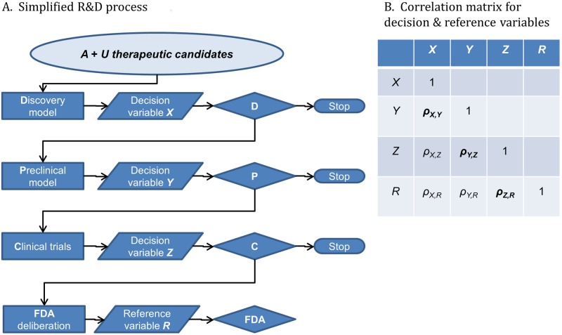
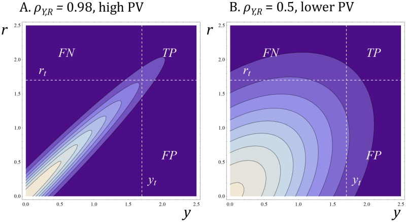
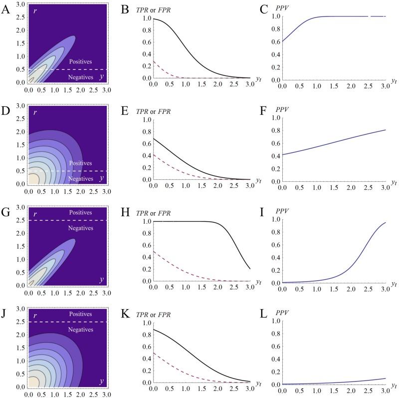
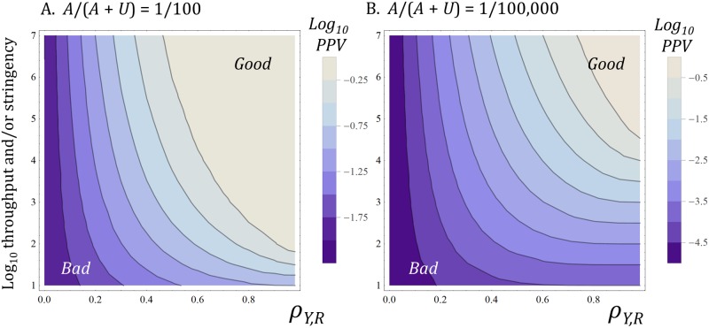
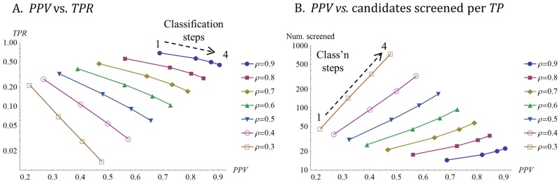
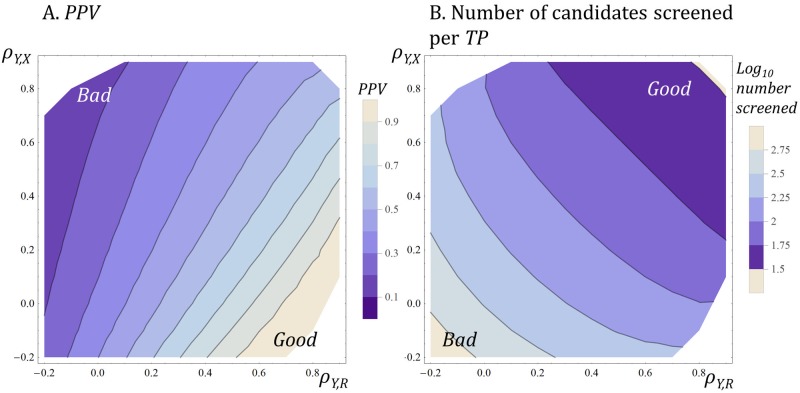
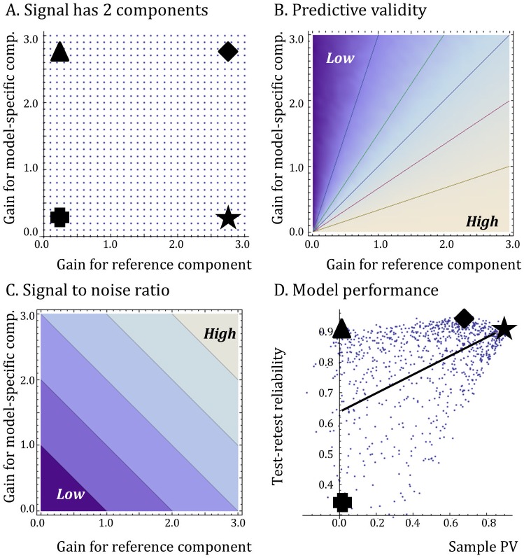
A striking contrast runs through the last 60 years of biopharmaceutical discovery, research, and development. Huge scientific and technological gains should have increased the quality of academic science and raised industrial R&D efficiency. However, academia faces a "reproducibility crisis"; inflation-adjusted industrial R&D costs per novel drug increased nearly 100 fold between 1950 and 2010; and drugs are more likely to fail in clinical development today than in the 1970s. The contrast is explicable only if powerful headwinds reversed the gains and/or if many "gains" have proved illusory. However, discussions of reproducibility and R&D productivity rarely address this point explicitly. The main objectives of the primary research in this paper are: (a) to provide quantitatively and historically plausible explanations of the contrast; and (b) identify factors to which R&D efficiency is sensitive. We present a quantitative decision-theoretic model of the R&D process. The model represents therapeutic candidates (e.g., putative drug targets, molecules in a screening library, etc.) within a "measurement space", with candidates' positions determined by their performance on a variety of assays (e.g., binding affinity, toxicity, in vivo efficacy, etc.) whose results correlate to a greater or lesser degree. We apply decision rules to segment the space, and assess the probability of correct R&D decisions. We find that when searching for rare positives (e.g., candidates that will successfully complete clinical development), changes in the predictive validity of screening and disease models that many people working in drug discovery would regard as small and/or unknowable (i.e., an 0.1 absolute change in correlation coefficient between model output and clinical outcomes in man) can offset large (e.g., 10 fold, even 100 fold) changes in models' brute-force efficiency. We also show how validity and reproducibility correlate across a population of simulated screening and disease models. We hypothesize that screening and disease models with high predictive validity are more likely to yield good answers and good treatments, so tend to render themselves and their diseases academically and commercially redundant. Perhaps there has also been too much enthusiasm for reductionist molecular models which have insufficient predictive validity. Thus we hypothesize that the average predictive validity of the stock of academically and industrially "interesting" screening and disease models has declined over time, with even small falls able to offset large gains in scientific knowledge and brute-force efficiency. The rate of creation of valid screening and disease models may be the major constraint on R&D productivity.

Fig 1. Decision theoretic view of biopharma discovery, research, and development.

(A) The process starts with a large set of therapeutic possibilities (light blue oval). These could be putative disease mechanisms or candidate drug targets, in either an academic or commercial setting. However, we discuss them as if they are molecules in a commercial R&D campaign (e.g., compounds in a screening library and the analogues that could be reasonably synthesized to create leads). There are A candidates that with perfect R&D decision making and an unlimited R&D budget would eventually be approved by the drug regulator for the indication or indications. There are U candidates that would not succeed given similar skill and investment. In general, U >> A. The Discovery (D), Preclinical (P), and Clinical Trial (C) diamonds are “classifiers” (Table 1). Each takes decision variables (X, Y, Z) from predictive models for some or all of the candidates and tests the variables against a decision threshold, yielding yeses which receive further scrutiny or noes which are abandoned. The unit cost per surviving candidate increases through the process [21]. Given serial decisions, only yeses from C face the gold standard reference test; the drug regulator (e.g., the Food and Drug Administration, or FDA). The other decisions face “imperfect” reference tests [33] [34] [27], the next steps in the process, which are mere proxies for the gold standard. The imperfect reference test for yeses from D is provided by P. The imperfect reference test for yeses from P is provided by C. (B) Decision variables X, Y, and Z, will correlate to a greater or lesser extent with each other and with the gold standard reference variable R. The correlation coefficient between X and Y is ρ_X,Y, the correlation coefficient between Y and Z is ρ_Y,Z, etc. Most of these correlations will never be measured directly during the R&D process. If ρ_X,R is very low, the Discovery stage will not enrich the Preclinical stage for approvable candidates, even if ρ_X,Y is high and decisions from D initially appear to have been successful.

Fig 2. Quantitative classifier model.

Bivariate normal probability density function determined by the correlation, ρ_Y,R, between decision variable, Y, and reference variable, R. Lighter colours indicate high probability density (candidate molecules more likely to lie here), and darker colours indicate a low probability density (molecules less likely to lie here). The units on the horizontal and vertical axes are one standard deviation. We apply a decision threshold, y_t (vertical dotted line) to the decision variable and then apply a reference test and a reference threshold, r_t,(horizontal dotted line) to molecules that exceed the decision threshold y_t. In the sensitivity analyses (see later) decision and reference thresholds are varied as is ρ_Y,R. True positives (TP) and false positives (FP) correspond to the probability mass in the upper right and lower right quadrants, respectively. (A) When ρ_Y,R is high, PPV is high. (B) When ρ_Y,R is low, PPV tends to be low.

Fig 3. Predictive validity and classifier performance.

(A) The bivariate normal probability density function for decision variable Y (horizontal axis) and reference variable R (vertical axis). The correlation between Y and R is high (ρ_Y,R = 0.95) so the decision variable has high PV. The graph shows only the positive quadrant of the distribution. The reference threshold, expressed here in units of standard deviation, is r_t = 0.5 (dotted line) so positives are common, accounting for P(R ≥ r_t) ≈ 30% of the probability mass. (B) shows TPR (solid line) and FPR (dotted line) as the decision threshold, y_t, varies. At some thresholds, the spread between the TPR and FPR is wide. (C) shows PPV vs. decision threshold, y_t. (D) to (F) repeat the analyses with a decision variable with lower PV (ρ_Y,R = 0.4). PPV declines vs. panel (C) but PPV remains high because positives are common. (G) to (I) repeat that analysis at ρ_Y,R = 0.95 but with a high reference threshold (2.5 standard deviation units) and rare positives (P(R ≥ r_t) ≈ 0.6% of the probability mass). It is possible to achieve a high PPV, but only at a high decision threshold when the TPR is low, which would require screening a large number of items per positive detected. (J) to (L) show the situation with the same high reference threshold (i.e., rare positives) but with a decision variable with low PV. In this case, PPV is low, even with a very high decision threshold and a very low TPR.

Fig 4. Decision performance as y_t (throughput) and ρ_Y,R (predictive validity) vary.

Shading shows the PPV of the classifier (log₁₀ units, with lighter shades showing better performance). The vertical axis represents both decision threshold and screening throughput. The scale is in log₁₀ units. 7 represents a throughput of 10⁷ and a decision threshold that accepts only the top 10^7th of candidates (P(Y ≥ y_t) = 10⁻⁷, Eq 6); 6 represents a throughput of 10⁶ and a decision threshold that accepts only the top 10^6th of candidates (P(Y ≥ y_t) = 10⁻⁶, Eq 6); etc. The horizontal axis represents PV as the correlation coefficient, ρ_Y,R, between Y and R, with the right hand end of each axis representing high PV (ρ_Y,R = 0.98), and the left hand end of each axis representing low PV (ρ_Y,R = 0). Our choice of scale for each axis is discussed in the main text. In (A), positives are relatively common. Here, P(R ≥ r_t) = 0.01, or one percent of the candidates entering the classifier. In (B), positives are relatively rare. Here, P(R ≥ r_t) = 10⁻⁵, or one hundred thousandth of the candidates entering the classifier. The spacing and orientation of the contours show the degree to which PPV changes with throughput and with ρ_Y,R. PPV is relatively sensitive to throughput when ρ_Y,R is high and when positives are very rare (lower right hand side of panel B.). However, PPV is relatively insensitive to throughput when ρ_Y,R is low (left hand side of both panels). For much of the parameter space illustrated, an absolute 0.1 change in ρ_Y,R (e.g., from 0.4 to 0.5, or 0.5 to 0.6 on the horizontal axis) has a larger effect on PPV than a 10x change in throughput (e.g., from 4 log₁₀ units to 5 log₁₀ units on the vertical axis).

Fig 5. Effect of multiple classification steps.

(A) Points represents decision performance with one, two, three, or four, similar classifiers applied in series. Each line represents the same value of correlation coefficient, ρ, applied to all pairwise relationships between decision variables and between decision variables and R. Thus in each line, all decision variables are equally correlated with each other and with R. The correlation coefficient between decision variables (X, Y, W, Z) and R vary from 0.9 (high PV, top right line) to 0.3 (low PV, bottom left line). The top left point on each line shows a single classifier applied to X, with each additional point towards the bottom and right of each line showing the effects of adding an additional classifier, up to a maximum of 4 classifiers. The top decile of candidates in the starting set exceed each decision threshold and the reference threshold (i.e., P(X ≥ x_t) = P(Y ≥ y_t) = P(W ≥ w_t) = P(Z ≥ z_t) = P(R ≥ r_t) = 0.1). In general, adding more steps increases PPV but at the cost of a lower TPR. There are diminishing returns from each additional classifier, particularly when the decision variables are highly correlated with one another. Furthermore, a single classifier that is highly correlated with R (e.g., the uppermost points on the lines with high correlation coefficients) often outperforms a combination of several classifiers with lower correlations with R in terms of both PPV and TPR. Note the logarithmic vertical axis. (B) is exactly as (A) but shows on the vertical axis the number of candidates screened per TP (Table 1). The number of candidates that must be screened per true positive identified increases as ρ (PV) declines because positives are wrongly rejected. Increasing ρ (PV) increases search efficiency. Note the logarithmic vertical axis.

Fig 6. Decision performance as correlations between decision variables change.

The first decision variable was X, and the correlation coefficient between X and R, ρ_X,R, was held constant at 0.5. The second decision variable was Y which varied in terms of its correlation with X (ρ_Y,X, vertical axes) and with reference variable R (ρ_Y,R, horizontal axes). Some regions of the graphs are empty because certain combinations of correlation coefficients cannot coexist. The top decile of candidates in the starting set exceed each decision threshold and the reference threshold (i.e., P(X ≥ x_t) = P(Y ≥ y_t) = P(R ≥ r_t) = 0.1). (A) shows PPV. Lighter shades indicate higher PPV. PPV increases as ρ_Y,R increases and as ρ_Y,X declines. The use of Y may depress PPV if Y is highly correlated with X while having a low correlation with R. (B) shows the number of candidates screened per TP. Darker shades indicate fewer candidates per TP. Note the log₁₀ colour scale. The number increases as ρ_Y,R declines and as ρ_Y,X declines.

Fig 7. Link between validity and reproducibility across a set of screening and disease models.

The figure shows the results of a Monte Carlo simulation (see S1 File for code). (A) Each small point represents one simulated screening or disease model (PM). When testing therapeutic candidates, each PM yields an expected signal which is the sum of two components. The first component is the signal from the reference test multiplied by a gain parameter (horizontal axis). The second component is a model-specific signal, whose gain is shown on the vertical axis. This component can also be thought of as systematic model-specific bias. It is real, but it tells us nothing about the reference test. (B) Each model’s PV is determined by the relative strength of the reference component versus the model-specific component of the signal. PV is high when the reference component is much larger than the model-specific component of the signal. This is because the output of the PM will correlate with the reference test when its signal is dominated by the reference signal. (C) Each PM’s signal to noise ratio increases with the sum of the reference component and the model-specific component. (D) Each point represents the performance of one of the models in Panel A., in two simulated experiments that include sampling and measurement noise. The horizontal axis shows the results of the first experiment. It is sample predictive validity (the correlation coefficient between the output of the model and the output of the reference test for a sample of therapeutic candidates). The vertical axis is the second experiment. It is test-retest reliability using the same sample of therapeutic candidates (calculated as the correlation coefficient between the results of the test and retest). The symbols (star, diamond, triangle, and cross) show how the space in (A) maps onto the space in (D). The line in (D) shows the best fit for the linear regression between sample PV and test-retest reliability. For the simulation shown, we sampled 400 therapeutic candidates for each PM. Both the reference and model-specific components of PM’s signal were drawn from a normally distributed random variable, whose mean was zero and whose standard deviations were equal to the respective gains on the horizontal and vertical axes of (A) to (C).

References

1. Scannell J, Blanckley A, Boldon H, Warrington B. Diagnosing the decline in pharmaceutical R&D efficiency. Nat Rev Drug Discov. 2012; 11: p. 191–200. 10.1038/nrd3681 - DOI - PubMed
1. Hogan JC. Combinatorial chemistry in drug discovery. Nat Biotechnol. 1997; 15: p. 328–330. - PubMed
1. Geysen HM, Schoenen F, Wagner D, Wagner R. Combinatorial compound libraries for drug discovery: an ongoing challenge. Nat Rev Drug Discov. 2003; 2: p. 222–230. - PubMed
1. Nature Biotechnology. Combinatorial chemistry. Nat Biotechnol. 2000; 18 supplement: p. IT50–IT52. - PubMed
1. Dolle RE. Historical overview of chemical library design In Zhou JZ, editor. Chemical Library Design (Methods in Molecular Biology 685).: Springer Science; 2011. p. 3–25. - PubMed
Publication types