Human Superior Temporal Gyrus Organization of Spectrotemporal Modulation Tuning Derived from Speech Stimuli

Abstract

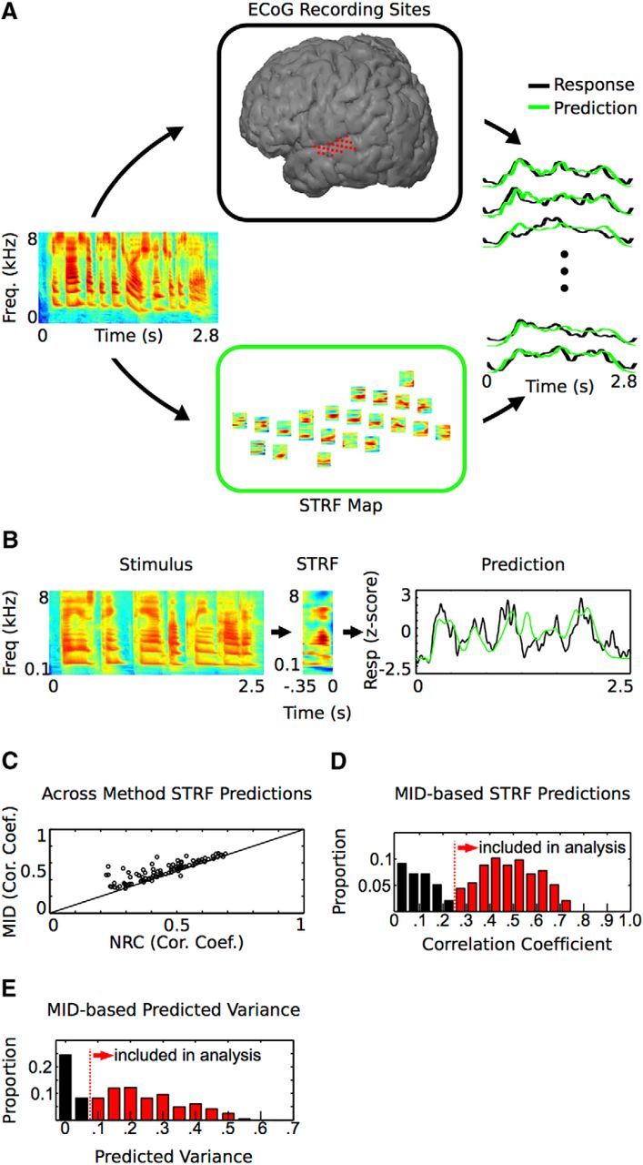
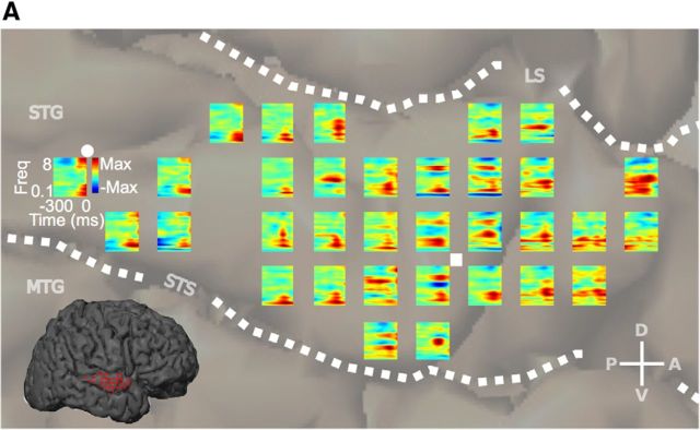
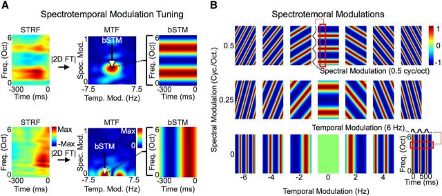
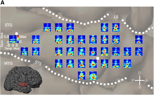
The human superior temporal gyrus (STG) is critical for speech perception, yet the organization of spectrotemporal processing of speech within the STG is not well understood. Here, to characterize the spatial organization of spectrotemporal processing of speech across human STG, we use high-density cortical surface field potential recordings while participants listened to natural continuous speech. While synthetic broad-band stimuli did not yield sustained activation of the STG, spectrotemporal receptive fields could be reconstructed from vigorous responses to speech stimuli. We find that the human STG displays a robust anterior-posterior spatial distribution of spectrotemporal tuning in which the posterior STG is tuned for temporally fast varying speech sounds that have relatively constant energy across the frequency axis (low spectral modulation) while the anterior STG is tuned for temporally slow varying speech sounds that have a high degree of spectral variation across the frequency axis (high spectral modulation). This work illustrates organization of spectrotemporal processing in the human STG, and illuminates processing of ethologically relevant speech signals in a region of the brain specialized for speech perception.

Significance statement: Considerable evidence has implicated the human superior temporal gyrus (STG) in speech processing. However, the gross organization of spectrotemporal processing of speech within the STG is not well characterized. Here we use natural speech stimuli and advanced receptive field characterization methods to show that spectrotemporal features within speech are well organized along the posterior-to-anterior axis of the human STG. These findings demonstrate robust functional organization based on spectrotemporal modulation content, and illustrate that much of the encoded information in the STG represents the physical acoustic properties of speech stimuli.

Keywords: functional organization; human STG; human superior temporal gyrus; modulation tuning; modulotopic; spectrotemporal processing.

Figure 1.

Experimental approach and the STRF. A, Experimental approach. An STRF was computed off-line for each ECoG electrode site (top, center) to generate a corresponding STRF map (bottom, center). The STRF describes the spectrotemporal structure in the stimulus that drives activity at a particular site. On the right is a subset of measured and predicted responses for the sentence “He sized up the situation and shook his head” (spectrogram at left). B, An STRF and the predicted and measured response for a single sentence. Predicted responses are obtained by convolving the stimulus with the STRF and are proportional to the similarity between the spectrotemporal content in the stimulus and the receptive field. C, Comparison of two methods used to compute STRFs. MID-based STRFs show higher predictive performance compared with normalized reverse correlation (NRC)-based STRFs (mean percentage increase in prediction: 19.0 ± 1.9% SEM, p < 0.001, Wilcoxon signed-rank test). D, MID-STRF Pearson correlation coefficient prediction values for all STG sites. E, MID-STRF predicted variance values for all sites. Sites with >5% of the variance predicted (red) were included in the analysis. MID, maximally informative dimension analysis; NRC, normalized reverse correlation analysis.

Figure 2.

Participant EC6 cortical STRF map. A, STRF map for participant EC6 (STRFs calculated with MID analysis). STG STRFs showed clear contiguous excitatory and inhibitory regions and structure characteristic of STRFs found in other regions. Representative temporal STRFs (•, tuned to quick onsets or offsets), and spectral STRFs (■, tuned to constant sound energy that fluctuates across frequency), are shown. LS, Lateral sulcus; STS, superior temporal sulcus; MTG, medial temporal gyrus; CS, central sulcus.

Figure 3.

The modulation transfer function and best spectrotemporal modulation (bSTM). A, Computation of the modulation transfer function (MTF). The MTF is derived as the magnitude of the two-dimensional Fourier transform of the STRF. It characterizes spectrotemporal modulation tuning for each site. Like the BF of a frequency tuning curve, the peak of the MTF defines the bSTM and represents a good descriptor of the overall MTF given the localized nature of modulation tuning within each MTF. For the site with the STRF shown at the top, the MTF indicates that high spectral modulations and low temporal modulations drive activity at that site. In contrast, the site below has a bSTM at high temporal modulations and low spectral modulations, indicating that the site is driven by changes in temporal and not spectral energy. B, Ordered array of spectrotemporal modulations as a function of their temporal and spectral modulation parameters. Spectrotemporal modulations represent the envelope “frequency” components of the spectrogram. Any spectrogram can be reconstructed exactly by a weighted sum of spectrotemporal modulations since they form a complete orthonormal basis of functions.

Figure 4.

Participant EC6 cortical modulation tuning map. A, Modulation tuning map for participant EC6. Each MTF is derived from the corresponding STRF. Representative temporal (•) and spectral (■) MTFs are shown. Although MTFs and STRFs contain equivalent information about spectrotemporal processing (except for phase information, which is discarded in MTFs), the overall structure of MTFs is less complex than that of STRFs. As shown, sites in the posterior STG are tuned for high temporal modulations (energy shifted away from the vertical midline) and sites in the anterior STG are tuned for slow temporal modulations and high spectral modulations (energy falling along the vertical midline and shifted upward). LS, Lateral sulcus; STS, superior temporal sulcus; MTG, medial temporal gyrus; CS, central sulcus.

Figure 5.

Organization of MTFs in STG. A, K-means cluster centroids generated from all MTFs across all participants. Their respective 50% contours are shown below. The overall tuning within an individual MTF centroid is fairly well localized. The collection of MTF centroid types span modulation space from high spectral/low temporal regions (red, left) to high temporal/low spectral regions (yellow, right) as shown by the 50% contours. B, Group MTF map. The map represents the average MTF across participants at each STG position. Only locations with ≥2 MTFs contributing to the average are included. Each MTF within the map is color-coded by its cluster membership. C, MTF cluster identity map. MTF cluster identities from B are plotted. The cluster identity map shows a transition from high spectral/low temporal MTFs anteriorly (red) to high temporal/low spectral MTFs posteriorly (yellow) and a significant degree of local organization (p < 1.0 × 10⁻⁵, neighborhood similarity permutation test). D, Average MTF cluster distance along the anterior–posterior extent of STG. Distances are measured from the anterior temporal pole illustrated in C (red horizontal axis). High spectral/low temporal MTFs are located anteriorly (red). High temporal/low spectral MTFs are located posteriorly (yellow, error bars represent SEM). E, Ensemble MTF (population average) for STG. Contour lines represent percentage maximum. LS, lateral sulcus; STG, superior temporal gyrus; MTG, medial temporal gyrus; CS, central sulcus.

Figure 6.

Organization of bSTM tuning in STG. A, bSTM tuning values from all participants. The distribution of bSTM values shows a particular relationship in which spectral modulation tuning decreases as temporal modulation tuning increases. B, Individual subject bSTM maps (A, color scale). Most participants show high temporal/low spectral modulation tuning posteriorly (blue), and high spectral/low temporal modulation tuning anteriorly (green) with significant nonrandom organization (EC6, p < 1.0 × 10⁻⁵; GP31, p = 5.0 × 10⁻⁴; EC36, p = 0.029; EC28, p = 4.5 × 10⁻⁵; EC53, p = 0.015; EC58, p = 0.10; EC56, p = 0.06; EC2, p = 0.42; two-parameter neighborhood similarity permutation test). C, Topographic ECoG site distribution along the anterior–posterior/dorsal–ventral extent of the STG. An example of the coordinate system used to measure distances is shown in D (red axis). Distances along the long axis of STG are measured from the anterior temporal pole. Distances along the short axis of STG are measured from the dorsal–ventral midpoint of the STG. D, Group spectrotemporal modulation tuning map. Only sites with data from ≥2 participants are included. High temporal/low spectral modulation tuned sites are located posteriorly (blue) and high spectral/low temporal modulation tuned sites are located anteriorly (green) with significant nonrandom organization and a mean gradient of +176° counterclockwise from the long axis of the STG (p < 1.0 × 10⁻⁵, neighborhood similarity permutation test). Data were binned at 4 × 4 mm resolution (same interelectrode distance as the ECoG array). E, Average best temporal modulation tuning as a function of distance along the dominant spectrotemporal modulation gradient. Individual subject maps were aligned by their gradients before averaging (blue, error bars represent SEM). Absolute distance is from the edge of data after maps have been aligned. The red function represents the raw average of temporal modulation tuning as a function of distance along the STG from the anterior temporal pole (D, horizontal red line; no map alignment by gradient before averaging). The inset represents data from normalized reverse correlation-based STRFs. F, Average best spectral modulation tuning as a function of distance along the dominant spectrotemporal modulation gradient. Maps were aligned by their gradients before averaging (green, error bars represent SEM). Absolute distance is from the edge of data after maps have been aligned. The red function represents the raw average of spectral modulation as a function of distance along the STG from the anterior temporal pole (D, horizontal red line; no map alignment by gradient before averaging). The inset represents data from normalized reverse correlation-based STRFs. LS, Lateral sulcus; STS, superior temporal sulcus; MTG, medial temporal gyrus; CS, central sulcus.

Figure 7.

DMR stimuli do not activate STG as robustly as speech stimuli from TIMIT. A, Spectrogram of a 3 s segment of the 5 min DMR stimulus (top) and examples of corresponding Z-scored high-gamma responses from STG electrodes in one subject (GP31). Z-score was calculated using a silent baseline period. Electrode responses are colored according to their best spectral modulation (BSM) and best temporal modulation (BTM) as derived from TIMIT stimuli. As demonstrated in the bottom panel, STG electrodes showed responses to the onset of DMR stimuli, but did not elicit strong responses during the rest of the 5 min stimulus. B, Comparison between the average response to the DMR stimulus and the average response to TIMIT sentences for STG electrodes (N = 4 subjects: EC63, GP30, GP31, GP33). The response to speech was significantly higher than the response to DMR stimuli (speech vs DMR, p = 1 × 10⁻²⁶; speech vs DMR (speech modulations), p = 1.6 × 10⁻²⁵, Wilcoxon signed rank test, 198 STG electrodes). The average response was calculated across the entire DMR stimulus (labeled DMR) and across time points during which the DMR included modulations within the tuning range for STG (labeled speech modulations: spectral modulations, ≤1 cycle/octave; the absolute value of the temporal modulations, ≤3 Hz). Gray lines connect the mean response for the same electrode across stimuli; black line indicates the average. For both stimuli, Z-scored responses were recalculated using a silent baseline to allow for comparisons across stimuli.

Figure 8.

Topography of spectral tuning. A, STRF-BF group map (color scale in B; only sites with data from ≥2 subjects are shown). The BF gradient runs in the anteroventral direction at +193° counterclockwise from the 3 o'clock position. Neither group map shows significant local organization. (STRF-BF, p = 0.1; SRF-BF, p = 0.06; neighborhood similarity permutation test). B, Individual participant STRF-BF maps. Two of eight maps show significant local organization for both metrics (STRF-BF p/SRF-BF p: EC6, p = 0.12/0.23; GP31, p = 0.004/0.007; EC36, p = 0.10/0.04; EC28, p = 0.02/0.75; EC53, p = 0.29/0.13; EC58, p = 0.27/0.07; EC56, p = 0.39/0.20; EC2, p = 0.11/0.25; neighborhood similarity permutation test). C, STRF-BF as a function of distance. Absolute distance is from the edge of data after maps have been aligned by their dominant gradient (black). The red function represents the raw average of BFs as a function of distance along the STG from the anterior temporal pole (A, horizontal red line; no map alignment by gradient before averaging). D, Example SRF with the 50% maximum line (red). At 50% maximum, this SRF has four peaks. E, Average peak number as a function of percentage maximum. F, Distribution of neurons types, in terms of peak number, as a function of percentage maximum level. Color scale represents proportion of neurons. At 90% maximum, 72% of the SRFs are single peaked, 25% are double peaked, and 3% have three peaks. G, BF distribution. The concentration of BFs in the STG is <1000 Hz, which is consistent with STG's placement as a low-frequency region in larger-scale cochleotopic maps. LS, Lateral sulcus; STS, superior temporal sulcus; MTG, medial temporal gyrus; CS, central sulcus.

References

1. Atencio CA, Schreiner CE. Spectrotemporal processing in spectral tuning modules of cat primary auditory cortex. PloS One. 2012;7:e31537. doi: 10.1371/journal.pone.0031537. - DOI - PMC - PubMed
1. Atencio CA, Sharpee TO, Schreiner CE. Cooperative nonlinearities in auditory cortical neurons. Neuron. 2008;58:956–966. doi: 10.1016/j.neuron.2008.04.026. - DOI - PMC - PubMed
1. Baumann S, Griffiths TD, Sun L, Petkov CI, Thiele A, Rees A. Orthogonal representation of sound dimensions in the primate midbrain. Nat Neurosci. 2011;14:423–425. doi: 10.1038/nn.2771. - DOI - PMC - PubMed
1. Baumann S, Joly O, Rees A, Petkov CI, Sun L, Thiele A, Griffiths TD. The topography of frequency and time representation in primate auditory cortices. Elife. 2015:4. doi: 10.7554/eLife.03256. - DOI - PMC - PubMed
1. Binder JR, Rao SM, Hammeke TA, Frost JA, Bandettini PA, Hyde JS. Effects of stimulus rate on signal response during functional magnetic resonance imaging of auditory cortex. Brain Res Cogn Brain Res. 1994;2:31–38. doi: 10.1016/0926-6410(94)90018-3. - DOI - PubMed
Publication types