Review
. 2016 Feb 16:7:10646.
doi: 10.1038/ncomms10646.

Integrating geological archives and climate models for the mid-Pliocene warm period

Affiliations
Review

Integrating geological archives and climate models for the mid-Pliocene warm period

Alan M Haywood et al. Nat Commun. .

Abstract

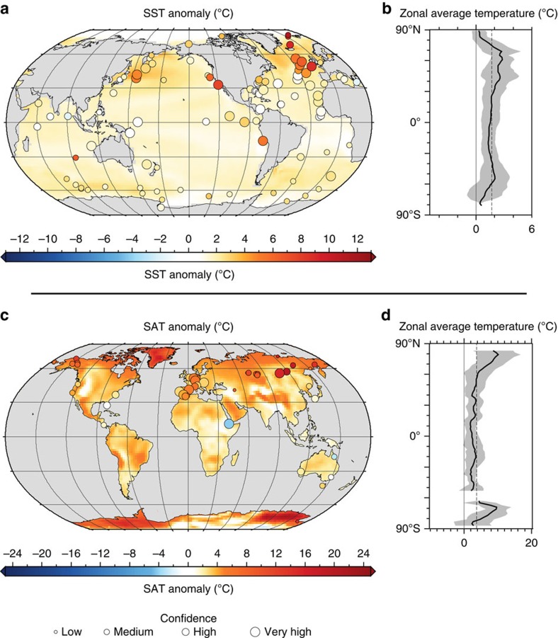
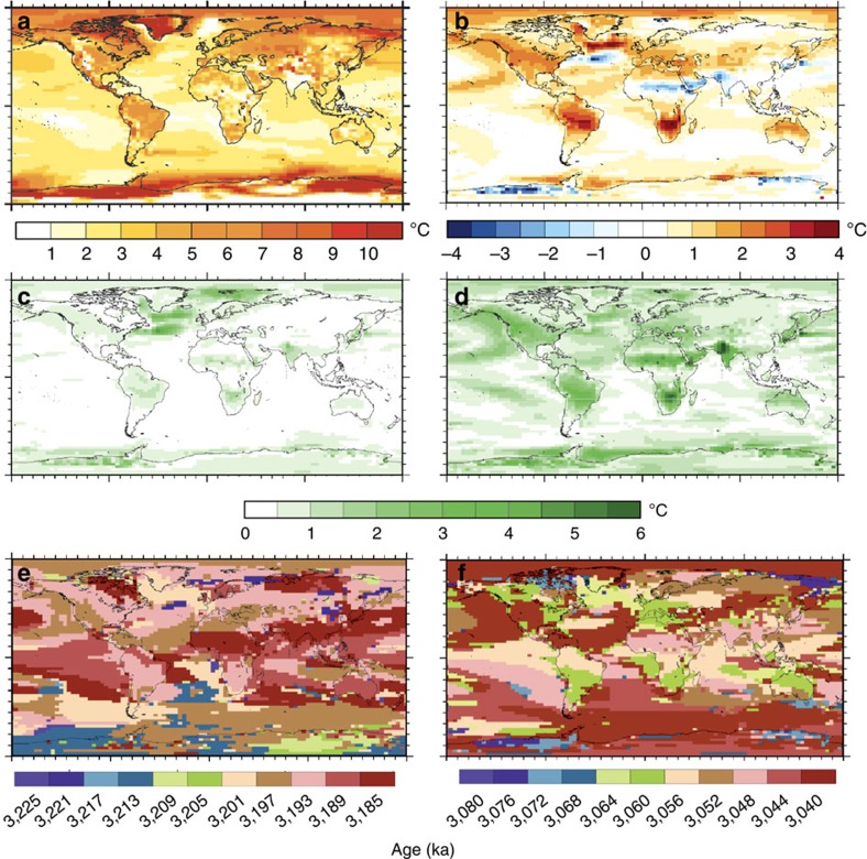
The mid-Pliocene Warm Period (mPWP) offers an opportunity to understand a warmer-than-present world and assess the predictive ability of numerical climate models. Environmental reconstruction and climate modelling are crucial for understanding the mPWP, and the synergy of these two, often disparate, fields has proven essential in confirming features of the past and in turn building confidence in projections of the future. The continual development of methodologies to better facilitate environmental synthesis and data/model comparison is essential, with recent work demonstrating that time-specific (time-slice) syntheses represent the next logical step in exploring climate change during the mPWP and realizing its potential as a test bed for understanding future climate change.


Figures

Figure 1
Figure 1. The Pliocene Research Interpretation and Synoptic Mapping Project Interval.
The PRISM interval in relation to the long-term climate evolution of the late Pliocene. (a) LR04 benthic oxygen isotope stack and timescale of Lisiecki and Raymo. Vertical dashed line shows present day δ18O value. The mPWP or PRISM3 warm interval (3.264–3.025 Ma) is shown by the horizontal shaded grey bar. (b) Laskar et al. values for obliquity (°), eccentricity and precession. (c) Details of LR04 timescale for the mPWP and position of PRISM4 and PlioMIP2 focus. Positions of Marine Isotope Stages MG1, M2, M1, KM5, KM3, KM2, KM1, K1, G21and G20 are shown.
Figure 2
Figure 2. Sample time series analyses.
Time series illustrating commonly used palaeoenvironmental proxies. Vertical grey band represents position of mPWP. (a) Equatorial Atlantic SST based on alkenone unsaturation index. (b) Caribbean Sea oxygen isotope record showing increasing salinity due to shoaling of the Central American Seaway. (c) Terrestrial record of the mean warmest month temperature from Lake El'gygytgyn. (d) Equatorial Pacific SST records based on Mg/Ca palaeothermometry. (e) Estimates of Pliocene atmospheric CO2 with pre-industrial and present day levels (horizontal dashed lines) for comparison; dark blue dots, δ13C (ref. 3); green band, δ11B (ref. 7); pink band, alkenone; red band, alkenone; orange band, stomata; yellow band, δ11B (ref. 5); blue band, Ba/Ca; Modified from ref. .
Figure 3
Figure 3. Evolution of the PRISM reconstruction.
The PRISM mean annual SST anomalies. (a) PRISM0 Northern Hemisphere reconstruction. (b) PRISM2 global reconstruction. (c) PRISM3 confidence-assessed global reconstruction where larger diameter circles represent higher confidence levels; numbers designate sample localities. SST anomaly colour scale the same for b,c.
Figure 4
Figure 4. Evolution of climate simulations.
Pliocene surface air temperature simulations. (a) Goddard Institute for Space Studies (GISS) Atmosphere-only climate model with PRISM prescribed boundary conditions. (b) Hadley Coupled Climate Model Version 3 simulation initiated with PRISM2 boundary conditions. (c) Community Climate Model Version 4 simulation initiated with PRISM3D boundary conditions.
Figure 5
Figure 5. Comparison of Data and Models.
International Panel on Climate Change (IPCC) data model comparison. Comparison of PRISM proxy data and the PlioMIP multimodel mean (MMM) simulation, (a) circles are PRISM SST anomalies, (b) zonally averaged PlioMIP MMM SST anomalies, (c) circles are PRISM land surface air temperature (SAT) anomalies, (d) zonally averaged MMM SAT anomalies. Zonal MMM gradients (b,d) are plotted with a shaded band indicating 2σ. Site-specific temperature anomalies estimated from PRISM proxy data are calculated relative to present site temperatures and are plotted (a,b) using the same colour scale as the model data, and a circle-size scaled to estimates of data confidence. Modified from Box 5.1, Fig. 1,.
Figure 6
Figure 6. Simulating Pliocene climate variability.
Hadley Coupled Climate Model Version 3 (HadCM3) simulations of surface air temperature (SAT °C) variability during the Pliocene redrawn and modified from ref. . (a) Annual mean Pliocene SAT (°C) prediction for interglacial Marine Isotope Stage (MIS) KM5c minus a pre-industrial experiment. (b) Annual mean SAT for Interglacial MIS K1 minus KM5c. Note that MIS K1 shows warmer SATs in most regions of the world compared to KM5c. (c) Variability in SATs 20 Kyrs ± of the benthic oxygen isotope peak of the KM5c interglacial. (d) Same as c but showing SAT variability ±20 Kyrs around the benthic oxygen isotope peak of the K1 interglacial. Note the larger degree of SAT variability in d compared to c. (e) Timing of the maximum SAT warming relative to the pre-industrial in each model grid box for KM5c ± 20 Kyrs. (f) Same as e but for K1 ±20 Kyrs. e and f Maximum SAT warming relative to the pre-industrial is not globally synchronous and varies in nature between MIS KM5c and K1. Modified from ref. .

Similar articles

Cited by

References

    1. IPCC. Climate Change 2013: The Physical Science Basis Contribution of Working Group I to the Fifth Assessment Report of the Intergovernmental Panel on Climate Change (eds Stocker T. F.et al.. 1535Cambridge University Press (2013).
    1. Valdes P. Built for stability. Nat. Geosci. 4, 414–416 (2011).
    1. Raymo M., Grant B., Horowitz M. & Rau G. Mid-Pliocene warmth: stronger greenhouse and stronger conveyor. Mar. Micropaleontol. 27, 313–326 (1996).
    1. Kürschner W. M., van der Burgh J., Visscher H. & Dilcher D. L. Oak leaves as biosensors of late Neogene and early Pleistocene paleoatmospheric CO2 concentrations. Mar. Micropaleontol. 27, 299–312 (1996).
    1. Seki O. et al.. Alkenone and boron-based Pliocene pCO2 records. Earth Planet. Sci. Lett. 292, 201–211 (2010).

Publication types

LinkOut - more resources