Predator-guided sampling reveals biotic structure in the bathypelagic

Abstract

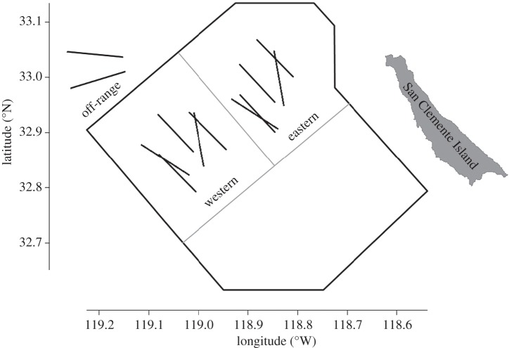
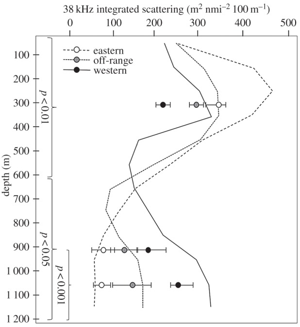
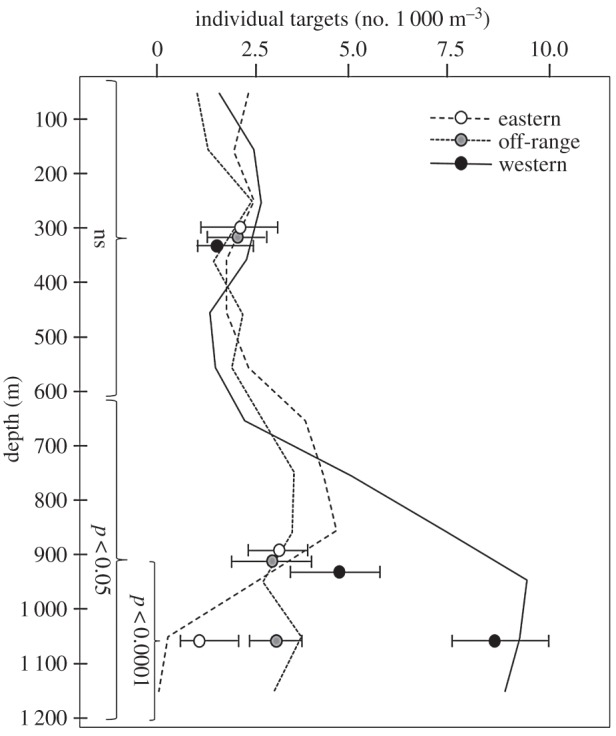
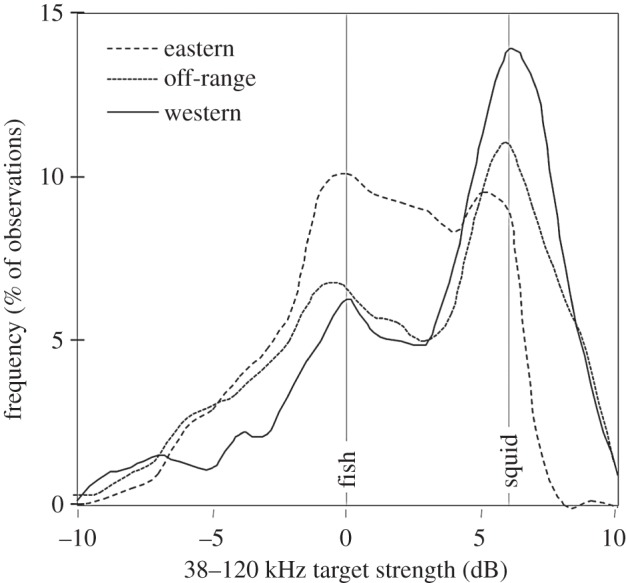
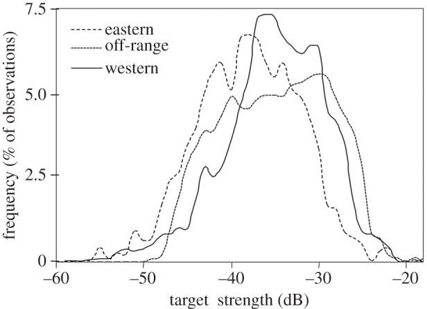
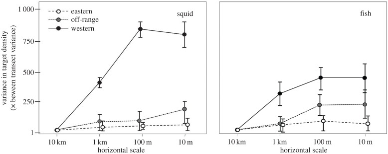
We targeted a habitat used differentially by deep-diving, air-breathing predators to empirically sample their prey's distributions off southern California. Fine-scale measurements of the spatial variability of potential prey animals from the surface to 1,200 m were obtained using conventional fisheries echosounders aboard a surface ship and uniquely integrated into a deep-diving autonomous vehicle. Significant spatial variability in the size, composition, total biomass, and spatial organization of biota was evident over all spatial scales examined and was consistent with the general distribution patterns of foraging Cuvier's beaked whales (Ziphius cavirostris) observed in separate studies. Striking differences found in prey characteristics between regions at depth, however, did not reflect differences observed in surface layers. These differences in deep pelagic structure horizontally and relative to surface structure, absent clear physical differences, change our long-held views of this habitat as uniform. The revelation that animals deep in the water column are so spatially heterogeneous at scales from 10 m to 50 km critically affects our understanding of the processes driving predator-prey interactions, energy transfer, biogeochemical cycling, and other ecological processes in the deep sea, and the connections between the productive surface mixed layer and the deep-water column.

Keywords: acoustics; deep sea; heterogeneity; pelagic; predator–prey.

Figure 1.

The locations of our sampling transects, each 10 km in length, are shown relative to the US Navy's SOAR range, outlined in black, off southern California. A priori Ziphius habitat use zones are delineated by grey lines to show a ‘high use’ zone in the northwest quadrant of the range and ‘low use’ in the northeast quadrant. Zones to the north of the range are the closest similar habitats that might be used by animals if range activities displace them.

Figure 2.

Acoustic scattering integrated over 100 m depth averaged over the transects in each zone is shown as a function of depth and sampling zone. In addition, integrations are shown for the upper 600 m of the water column, 600–1 200 m, and 900–1 200 m for each zone. Error bars show the total range of values for transects in that zone. Significance levels for post-hoc analysis of the effects of zone on extended integration depths are shown for each panel.

Figure 3.

The density of individual targets as a function of depth range and sampling zone is shown over 100 m depth bins. Values are shown averaged over the upper 600 m of the water column, 600–1 200 m, and 900–1 200 m for each zone. Error bars show the total range of values for transects in that zone. Significance levels for post-hoc analysis of the effects of sampling zone are shown for each panel.

Figure 4.

Smoothed histograms of the frequency response of individual targets detected between 900 and 1 200 m as a function of sampling zone. The expected frequency response for fish (0 dB) and squid (6 dB) are indicated by grey lines. The y-axis is the per cent of observations within each zone. This allows the relative proportion of different scatters to be observed across zones.

Figure 5.

Smoothed histograms of the target strength of targets consistent with squid for each of the three habitat use categories. The y-axis is the frequency measured as the per cent of observations within each category.

Figure 6.

To quantify the spatial distribution or patchiness of potential Ziphius prey over a range of scales, variance in the density of targets consistent with squid among segments of each transect was scaled by the between transect variance within each habitat use category as transects were split into smaller and smaller sections. Shown here are the data consistent with squid with error bars showing the variance in this measure between transects. Note that data from the eastern and off-range sampling zones are offset slightly for visual clarity however transect segments were not different in size.

References

1. Robison BH. 2004. Deep pelagic biology. J. Exp. Mar. Biol. Ecol. 300, 253–272. (10.1016/j.jembe.2004.01.012) - DOI
1. Backus R, Craddock J, Haedrich R, Robison B. 1977. Atlantic mesopelagic zoogeography. Fish. Western North Atlantic 7, 266–287.
1. Robison BH. 1995. Light in the ocean's midwaters. Sci. Am. 273, 60 (10.1038/scientificamerican0795-60) - DOI
1. Haedrich R. 1996. Deep-water fishes: evolution and adaptation in the earth's largest living spaces. J. Fish Biol. 49, 40–53. (10.1111/j.1095-8649.1996.tb06066.x) - DOI
1. Clarke MR. 1996. The role of cephalopods in the world's oceans: an introduction. Phil. Trans. R. Soc. Lond. B 351, 979–983. (10.1098/rstb.1996.0088) - DOI
Publication types