Temperature-driven global sea-level variability in the Common Era

Abstract

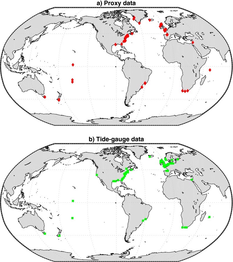
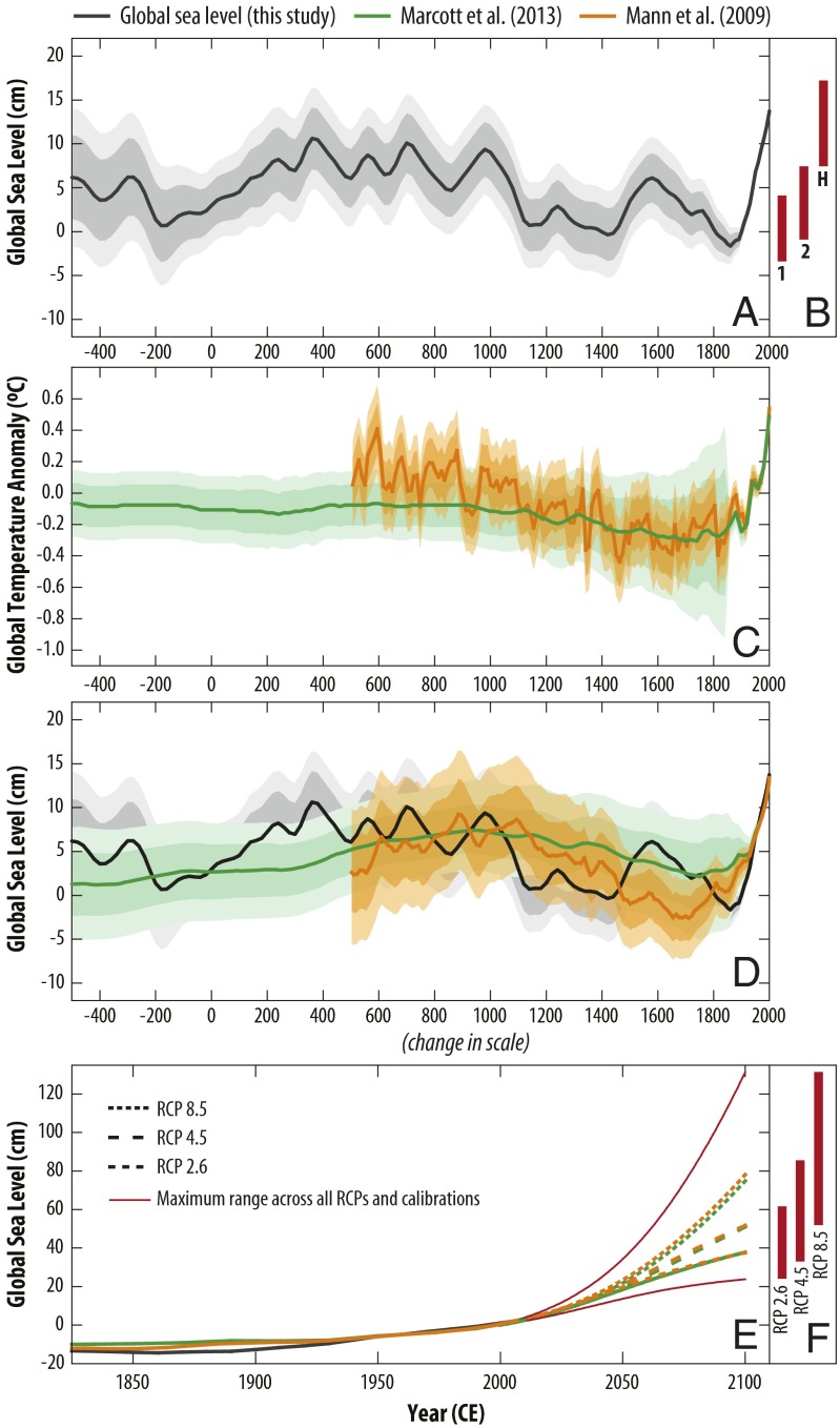
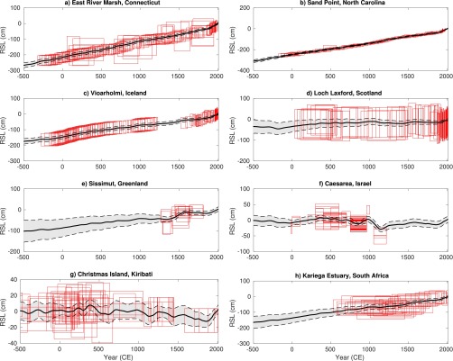
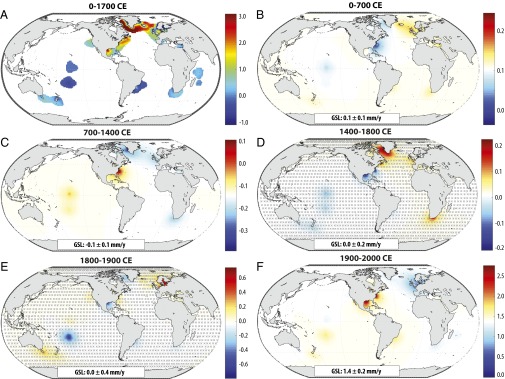
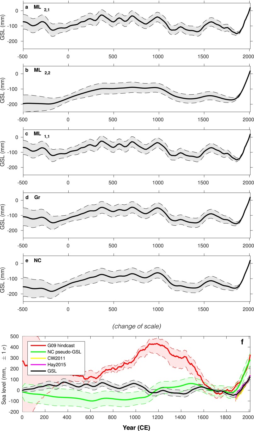
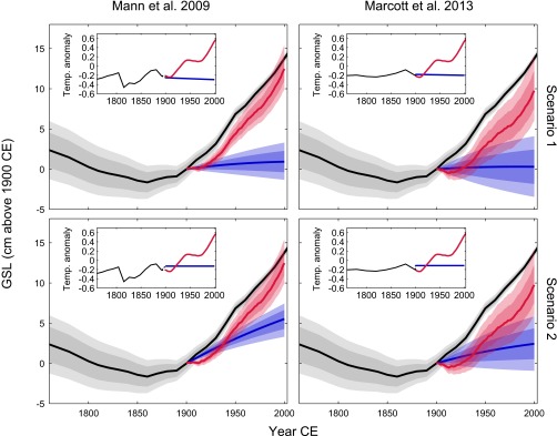
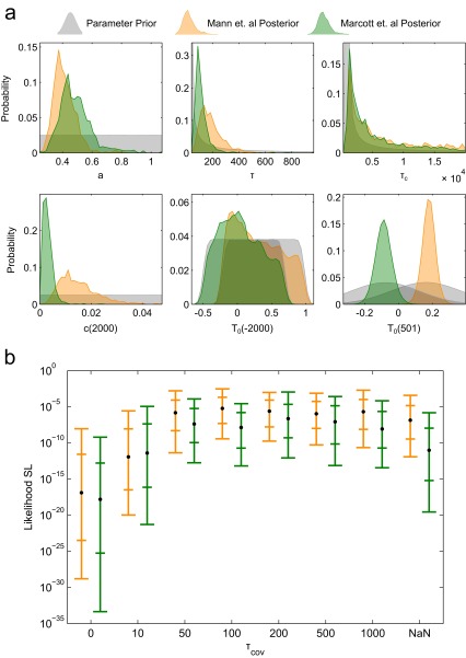
We assess the relationship between temperature and global sea-level (GSL) variability over the Common Era through a statistical metaanalysis of proxy relative sea-level reconstructions and tide-gauge data. GSL rose at 0.1 ± 0.1 mm/y (2σ) over 0-700 CE. A GSL fall of 0.2 ± 0.2 mm/y over 1000-1400 CE is associated with ∼ 0.2 °C global mean cooling. A significant GSL acceleration began in the 19th century and yielded a 20th century rise that is extremely likely (probability [Formula: see text]) faster than during any of the previous 27 centuries. A semiempirical model calibrated against the GSL reconstruction indicates that, in the absence of anthropogenic climate change, it is extremely likely ([Formula: see text]) that 20th century GSL would have risen by less than 51% of the observed [Formula: see text] cm. The new semiempirical model largely reconciles previous differences between semiempirical 21st century GSL projections and the process model-based projections summarized in the Intergovernmental Panel on Climate Change's Fifth Assessment Report.

Keywords: Common Era; climate; late Holocene; ocean; sea level.

Fig. S1.

Locations of sites with (A) proxy data and (B) tide-gauge data included in the analysis.

Fig. 1.

(A) Global sea level (GSL) under prior ML_2,1. Note that the model is insensitive to small linear trends in GSL over the Common Era, so the relative heights of the 300–1000 CE and 20th century peaks are not comparable. (B) The 90% credible intervals for semiempirical hindcasts of 20th century sea-level change under historical temperatures (H) and counterfactual scenarios 1 and 2, using both temperature calibrations. (C) Reconstructions of global mean temperature anomalies relative to the 1850–2000 CE mean (1, 2). (D) Semiempirical fits to the GSL curve using the two alternative temperature reconstructions. (E) As in B, including 21st century projections for RCPs 2.6, 4.5, and 8.5. Red lines show the fifth percentile of RCP 2.6 and 95th percentile of RCP 8.5. (F) The 90% credible intervals for 2100 by RCP. In A, B, and D, values are with respect to 1900 CE baseline; in E and F, values are with respect to 2000 CE baseline. Heavy shading, 67% credible interval; light shading, 90% credible interval.

Fig. S2.

Model fits under prior ML_2,1 at eight illustrative sites: (A) East River Marsh, CT; (B) Sand Point, NC, (C) Vioarholmi, Iceland, (D) Loch Laxford, Scotland, (E) Sissimut, Greenland, (F) Caesarea, Israel, (G) Christmas Island, Kiribati, and (H) Kariega Estuary, South Africa. (Note that the model fit at each site is informed by all observations, not just those at the illustrated site.) Red boxes show all data points within 0.1 degrees of the centroid of the named site. Errors are $\pm 2\sigma$.

Fig. 2.

(A) Mean estimated rate of change (millimeters per year) over 0–1700 CE under prior ML_2,1. In shaded areas, conditioning on the observations reduces the variance by at least 10% relative to the prior. (B−F) Mean estimated rates of change (mm/y) from (B) 0–700 CE, (C) 700–1400 CE, (D) 1400–1800 CE, (E) 1800–1900 CE, and (F) 1900–2000 CE, after removing the 0–1700 CE trend. Areas where a rise and a fall are about equally likely ($P=$ 0.33–0.67) are crosshatched. The color scales are centered around the noted rate of GSL change.

Fig. S3.

(A–E) GSL estimates under priors (A) ML_2,1, (B) ML_2,2, (C) ML_1,1, (D) Gr, and (E) NC. (F) GSL reconstruction under prior ML_2,1 (black) compared with the hindcast of ref. (G09 hindcast; red), a curve derived from the North Carolina RSL curve by detrending and the addition of $\pm 10$ mm ($2\sigma$) errors after ref. (NC pseudo-GSL; green), and the 19th–20th century GMSL reconstructions of ref. (Hay2015; magenta) and ref. (CW2011; yellow). Multicentury records are aligned relative to the 1600–1800 CE average; 19th–20th century reconstructions are aligned to match our GSL reconstruction in 2000 CE. Errors are $\pm 1\sigma$.

Fig. S4.

Counterfactual hindcasts of global mean sea-level rise in the absence of anthropogenic warming. Each row assumes a different counterfactual temperature scenario (see Materials and Methods), while each column represents model calibration to a different temperature reconstruction (Inset). In the temperature Insets, the black lines represent the original temperature reconstruction to 1900, the red line represents the HadCRUT4 temperature reconstruction for the 20th century, and the blue line represents the counterfactual scenario. In the main plots, the red and blue curves correspond, respectively, to the HadCRUT4 and counterfactual temperature scenarios. The difference between them can be interpreted as the anthropogenic GSL rise. Heavy shading, 67% credible; light shading, 90% credible.

Fig. S5.

(A) Probability distributions of semiempirical model parameters. Prior distributions (gray) are not shown in full where scaling axes to display them would render posteriors obscure. (B) Likelihood of different values of ${\tau }_{cov}$. Black dots show likelihoods across all semiempirical projections, and the bars show the 5th/17th/83rd/95th percentile conditional likelihoods for individual semiempirical projections. A value of ${\tau }_{cov}=100$ y is used in the analysis. Orange [green] represents calibration with the Mann et al. (1) [Marcott et al. (2)] temperature curve.

References

1. Mann ME, et al. Global signatures and dynamical origins of the Little Ice Age and Medieval Climate Anomaly. Science. 2009;326(5957):1256–1260. - PubMed
1. Marcott SA, Shakun JD, Clark PU, Mix AC. A reconstruction of regional and global temperature for the past 11,300 years. Science. 2013;339(6124):1198–1201. - PubMed
1. PAGES 2K Consortium Continental-scale temperature variability during the past two millennia. Nat Geosci. 2013;6(5):339–346.
1. Jevrejeva S, Grinsted A, Moore J. Anthropogenic forcing dominates sea level rise since 1850. Geophys Res Lett. 2009;36(20):L20706.
1. Kemp AC, et al. Climate related sea-level variations over the past two millennia. Proc Natl Acad Sci USA. 2011;108(27):11017–11022. - PMC - PubMed
Publication types
LinkOut - more resources