. 2016 Feb 25;12(2):e1004778.
doi: 10.1371/journal.pcbi.1004778. eCollection 2016 Feb.

Cell Assembly Dynamics of Sparsely-Connected Inhibitory Networks: A Simple Model for the Collective Activity of Striatal Projection Neurons

Affiliations

Cell Assembly Dynamics of Sparsely-Connected Inhibitory Networks: A Simple Model for the Collective Activity of Striatal Projection Neurons

David Angulo-Garcia et al. PLoS Comput Biol. .

Abstract

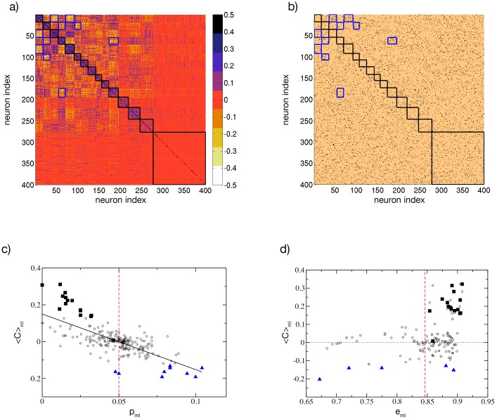
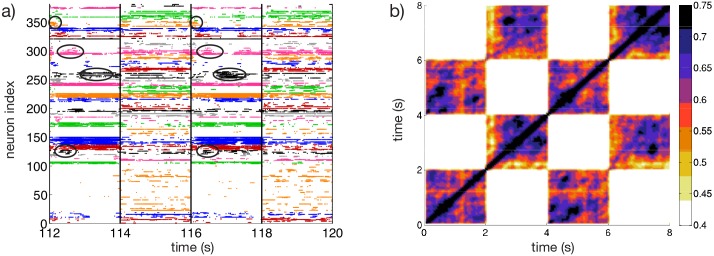
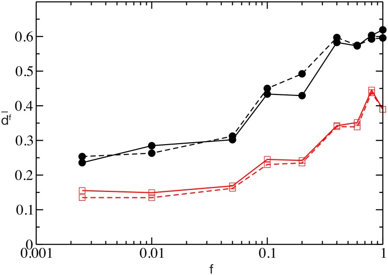
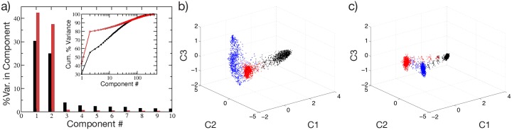
Striatal projection neurons form a sparsely-connected inhibitory network, and this arrangement may be essential for the appropriate temporal organization of behavior. Here we show that a simplified, sparse inhibitory network of Leaky-Integrate-and-Fire neurons can reproduce some key features of striatal population activity, as observed in brain slices. In particular we develop a new metric to determine the conditions under which sparse inhibitory networks form anti-correlated cell assemblies with time-varying activity of individual cells. We find that under these conditions the network displays an input-specific sequence of cell assembly switching, that effectively discriminates similar inputs. Our results support the proposal that GABAergic connections between striatal projection neurons allow stimulus-selective, temporally-extended sequential activation of cell assemblies. Furthermore, we help to show how altered intrastriatal GABAergic signaling may produce aberrant network-level information processing in disorders such as Parkinson's and Huntington's diseases.


Conflict of interest statement

The authors have declared that no competing interests exist.

Figures

Fig 1
Fig 1. Cell activity characterization.
a) Firing rates νi of 6 selected neurons belonging to two anti-correlated assemblies, the color identifies the assembly and the colors correspond to the one used in b) for the different clusters; b) raster plot activity, the firing times are colored according to the assembly the neurons belong to; c) cross-correlation matrix C(νi, νj) of the firing rates. The neurons in panel b) and c) are clustered according to the correlation of their firing rates by employing the k-means algorithm; the clusters are ordered in terms of their average correlation (inside each cluster) from the highest to the lowest one (for more details see Methods). The firing rates are calculated over overlapping time windows of duration 1 s, the origins of successive windows are shifted by 50 ms. The system is evolved during 107 spikes, after discarding an initial transient of 105 spike events. Other parameters used in the simulation: g = 8, K = 20, N = 400, kmean = Nact/15, ΔV = 5 mV and τα = 20 ms. The number of active neurons is 370, corresponding to n* ≃ 93%.
Fig 2
Fig 2. Metrics of structured activity vs lateral inhibition strength.
a) Metrics entering in the definition of Q0 versus the synaptic strength g. From top to bottom: Averaged coefficient of variation 〈CVN, standard deviation of the cross-correlation matrix σ(C), and the fraction of active neurons n*. The solid (dashed) line refers to the case ΔV = 1 mV (ΔV = 5 mV). The minimum number of active neurons is achieved at g = gmin, this corresponds to a peak amplitude of the PSP APSP = 0.064 mV (APSP = 0.184 mV) for ΔV = 1 mV (ΔV = 5 mV) (for more details see Methods). b) Distributions P(ISI¯) of the average ISI for a fixed ΔV = 5 mV and for two different coupling strengths, g = 4 (red triangle-up symbol) and g = 10 (blue triangle-down). Inset, the distribution P(CV) of the CV of the single neurons for the same two cases. c) Q0 and Qd, as defined in Eqs (1) and (20), versus g for ΔV = 1 mV. d) Same as c) for ΔV = 5 mV. Other parameters as in Fig 1.
Fig 3
Fig 3. Metrics of structured activity vs post-synaptic time duration.
a) Metrics Q0 (in solid line) and Qd (dashed) as a function of the pulse time scale for the parameter values {ΔV,g} = {5 mV,8} corresponding to the maximum Q0 value in Fig 2(d). Probability distribution functions P(CV) (P(CV2)) for the coefficient of variation CV (local coefficient of variation CV2) are shown in b) (in c)) for three representative τα = {2, 9, 20} ms, indicated in the three panels with red squares, blue triangles-up and black circles respectively. For these three cases the average firing rate in the network is 〈ν〉 = {8.81,7.65,7.35} Hz ordered for increasing τα-values. Other parameters as in Fig 1.
Fig 4
Fig 4. Single neuron statistics.
a) Distribution P(ISI) at short values of ISIs for one representative cell in the network, by setting τα = 20 ms. Inset: same as main figure for the whole range of ISIs. b) Same as a) for τα = 2 ms. c-d) Corresponding Poissonian reconstruction of the P(ISI) for the same cases depicted in a) and b). e-f) Single neuron distribution of the CV2(i) for the same considered cases as in a) and b) calculated from the simulation (black solid lines with circles) and the Poissonian reconstruction (red dashed line with squares). The network parameters are ΔV = 5 mV and g = 8, remaining parameters as in Fig 1. Both the examined neurons have Is = −45.64 mV. For the Poissonian reconstruction the frequencies of the incoming uncorrelated spike trains are set to 〈νN ≈ 7.4 Hz (〈νN ≈ 8.3 Hz) for τα = 20ms (τα = 2ms), as measured from the corresponding network dynamics. The distributions are obtained by considering a sequence of 109 spikes in the original network, and 107 events for the Poissonian reconstruction.
Fig 5
Fig 5. Cell assemblies and connectivity.
a) Cross-correlation matrix C(νi, νj) of the firing rates organized according to the clusters generated via the k-means algorithm with k = 15, the clusters are ordered as in Fig 1(c) from the highest to the lowest correlated one. b) Connectivity matrix Cij with the indices ordered as in panel a). Here, a black (copper) dot denotes a 1 (0) in Cij, i.e. the presence(absence) of a synaptic connection from j to i. c) Average cross-correlation 〈Cml among the elements of the matrix block (m, l), versus the probability pml to have synaptic connections from neurons in the cluster l to neurons in the cluster m. d) 〈Cml versus the block averaged similarity metrics eml. Black squares indicate the blocks along the diagonal delimited by black borders in panel a) and b); blue triangles denote the ten blocks with the lowest 〈Cml values, which are also delimited by blue edges in a) and b). The vertical red dashed line in panel c) denotes the average probability to have a connection p = 5% and in panel d) the value of the metrics eml averaged over all the blocks. The black solid line in panel c) is the linear regression to the data (〈Cml ≈ 0.15–3.02pml, correlation coefficient R = −0.72). Other parameters as in Fig 1.
Fig 6
Fig 6. Sequential switching.
a) Raster plot associated to the two input protocols I(1) and I(2). The circles denote the clusters of active neurons appearing repetitively after the presentation of the stimulus I(1). Vertical lines denote the switching times between stimuli. The clustering algorithm employed to identify the different groups is applied only during the presentation of the stimulus I(1), therefore the sequential dynamics is most evident for that particular stimulus. b) Averaged State Transition Matrix D¯, obtained by considering a 4Tsw × 4Tsw sub-matrix averaged over r = 5 subsequent time windows of duration 4Tsw (see the section Methods for details). The inputs I(1) and I(2) are different realization of the same random process, they are obtained by selecting N current values Ii from the flat interval [Vth, Vth + ΔV]. The input stimuli are switched every Tsw = 2 s. Number of clusters k = 35 in a). Other parameters as in Fig 1.
Fig 7
Fig 7. Pattern separation.
Average dissimilarity as a function of the fraction f of inputs differing from the control input, for the values of τα = 20ms (black circles) and τα = 2ms (red squares) with two different observation windows TE = 2s (solid line) and TE = 10s (dashed line). Other parameters used: ΔT = 50ms, ΔV = 5 mV. Remaining parameters as in Fig 1.
Fig 8
Fig 8. Computational capability of the network.
Characterization of the firing activity of the network, obtained as response to three consecutive inputs presented in succession. a) Percentage of the variance of the neuronal firing activity reproduced by each of the first 10 principal components. The inset displays the corresponding cumulative percentage as a function of the considered component. Filled black and shaded red (bar or symbols) correspond to τα = 20 ms and τα = 2 ms, respectively. Projection of the neuronal response along the first three principal components for b) τα = 20 ms and c) τα = 2 ms. Each point in the graph correspond to a different time of observation. The three colors denote the response to the three different inputs, which are quenched stimulation currents randomly taken as I(j) ∈ [Vth, Vth + ΔV] for j = 1, 2, 3, the experiment is then performed as explained in the text.
Fig 9
Fig 9. Response of the network to an increase in the excitability.
a,f) Network Bursting Rate, and the threshold defined for considering a synchronized event. b,g) Neurons involved in the synchronized events, vertical lines denoted the switching times between the excited I(e) and control I(c) inputs. Colors in the raster indicates the group assigned to the synchronous event using an optimal community partition algorithm. c,h) Synchronized Event Transition Matrix, calculated with a window TW = 50 ms and number of events Ss = 20. d,i) Projection of the synchronized events in the 2D space spanned by the first two principal components associated to the covariance matrix of the vectors Ws. e,j) Number of coactive cells in each state. The diagonal elements of the bar graph represents the total number of neurons contributing to one state. Panels (a-e) correspond to g = 8, while panels (f-j) depict the case g = 1. In both cases the system is recorded during the time span required to identify Ss = 20. Remaining parameters as in Fig 1.

References

    1. Stephenson-Jones M, Samuelsson E, Ericsson J, Robertson B, Grillner S. Evolutionary conservation of the basal ganglia as a common vertebrate mechanism for action selection. Current Biology. 2011;21(13):1081–1091. 10.1016/j.cub.2011.05.001 - DOI - PubMed
    1. Daw ND, Doya K. The computational neurobiology of learning and reward. Current opinion in neurobiology. 2006;16(2):199–204. 10.1016/j.conb.2006.03.006 - DOI - PubMed
    1. Merchant H, Harrington DL, Meck WH. Neural basis of the perception and estimation of time. Annual review of neuroscience. 2013;36:313–336. 10.1146/annurev-neuro-062012-170349 - DOI - PubMed
    1. Wilson CJ, Groves PM. Fine structure and synaptic connections of the common spiny neuron of the rat neostriatum: a study employing intracellular injection of horseradish peroxidase. Journal of Comparative Neurology. 1980;194(3):599–615. 10.1002/cne.901940308 - DOI - PubMed
    1. Groves PM. A theory of the functional organization of the neostriatum and the neostriatal control of voluntary movement. Brain Research Reviews. 1983;5(2):109–132. 10.1016/0165-0173(83)90011-5 - DOI - PubMed

Publication types

LinkOut - more resources