Continued emissions of carbon tetrachloride from the United States nearly two decades after its phaseout for dispersive uses

Abstract

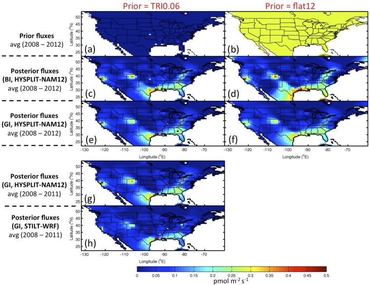
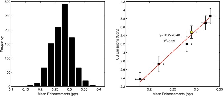
National-scale emissions of carbon tetrachloride (CCl4) are derived based on inverse modeling of atmospheric observations at multiple sites across the United States from the National Oceanic and Atmospheric Administration's flask air sampling network. We estimate an annual average US emission of 4.0 (2.0-6.5) Gg CCl4 y(-1) during 2008-2012, which is almost two orders of magnitude larger than reported to the US Environmental Protection Agency (EPA) Toxics Release Inventory (TRI) (mean of 0.06 Gg y(-1)) but only 8% (3-22%) of global CCl4 emissions during these years. Emissive regions identified by the observations and consistently shown in all inversion results include the Gulf Coast states, the San Francisco Bay Area in California, and the Denver area in Colorado. Both the observation-derived emissions and the US EPA TRI identified Texas and Louisiana as the largest contributors, accounting for one- to two-thirds of the US national total CCl4 emission during 2008-2012. These results are qualitatively consistent with multiple aircraft and ship surveys conducted in earlier years, which suggested significant enhancements in atmospheric mole fractions measured near Houston and surrounding areas. Furthermore, the emission distribution derived for CCl4 throughout the United States is more consistent with the distribution of industrial activities included in the TRI than with the distribution of other potential CCl4 sources such as uncapped landfills or activities related to population density (e.g., use of chlorine-containing bleach).

Keywords: United States; carbon tetrachloride; emissions; greenhouse gases; ozone-depleting substances.

Fig. 1.

Map showing the locations of flask air sampling sites where CCl₄ was measured as part of this study (aircraft, triangles; tall towers, stars), the resulting sensitivity of this sampling network to CCl₄ emissions throughout the United States during 2008–2012 (color shading from yellow to red), and the distribution of emissions reported by different facilities to the US EPA TRI (circles with size indicating emission magnitude). Sites excluded from the inversions and displayed surface sensitivity are indicated as unfilled triangles and stars. Two aircraft sampling sites are not apparent in this map: PFA (65.07°N, 147.29°W) and RTA (21.25°S, 159.83°W).

Fig. 2.

Measured atmospheric mole fractions of CCl₄ in different regions (A and B) and site-specific mole fraction enhancements above remote atmosphere or “background” values (measured at 3–6 km agl) (C), and over time in observations and in forward calculations using different emissions (D). Measured mole fractions in the free troposphere (3–6 km agl) (gray points) are very similar to those measured in the lower atmosphere (0–1 km agl) (black points) at remote sites upwind of the contiguous United States (THD, ESP, and ETL) (A); in the midcontinent, samples with CCl₄ mole fractions above background values are observed (B) (the few results above 110 ppt observed at midcontinent sites are not visible). The distribution of enhanced mole fractions measured near the surface (0–500 m agl) has significant spatial variability (C) likely indicative of spatial variations in emission strength (error bars represent the standard error of mean mole fraction enhancements, and site code + “a” indicates aircraft sites). (D) Observed (obs, black unfilled squares connected with a black line) and simulated (sim) monthly median mole fraction enhancements in the lower atmosphere (0–500 m agl) using emissions reported in the US EPA TRI (blue line) and posterior emissions derived here (red line with gray shading representing uncertainty of simulations).

Fig. S1.

A comparison of background and free tropospheric CCl₄ mole fractions from different regions and sampling programs. CCl₄ mole fractions in the free troposphere (3–6 km agl) at midcontinental nonremote sites as in Fig. 2 (gray) and remote sites upwind of the contiguous United States (THD, ESP, and ETL; blue), as well as those from the HIPPO campaign measured on the same GCMS instrument (red). CCl₄ mole fractions in the lower atmosphere (0–3 km agl) in the remote atmosphere are also shown as cyan (THD, ESP, and ETL) and yellow (HIPPO) symbols.

Fig. S2.

Observed average vertical gradients of CCl₄ at aircraft sites during 2008–2012. Error bars represent standard errors of average enhancements at different altitudes.

Fig. S3.

The distribution and magnitude of emissions used as priors and derived as posteriors from multiple approaches and input data to the inverse calculation. Prior emissions were from the US EPA TRI, which yielded an average national total emission of 0.06 Gg⋅y⁻¹ during 2008–2012 (TRI0.06 in A), and a spatially flat prior with a constant national total emission of 12 Gg⋅y⁻¹ (flat12 in B). Posterior emissions of CCl₄ averaged over 2008–2012 were derived with a Bayesian inverse analysis (BI) and air transport simulated by HYSPLIT-NAM12 and the different priors (TRI0.06 in C and flat12 in D); they were also derived with the same representation of transport and a Geostatistical inverse analysis (GI) and the different priors (TRI0.06 in E and flat12 in F). Finally, the influence of a different approach to simulating transport (STILT-WRF) is apparent in the comparison of derived emissions averaged over a subset of years (2008–2011), the TRI0.06 prior, and a GI approach using HYSPLIT-NAM (G) or STILT-WRF (H).

Fig. 3.

The magnitude and distribution of annual CCl₄ emissions derived for the contiguous United States in this study from a flat prior (flat12) (A) and reported to the US EPA TRI (B) averaged over 2008–2012 (displayed as annual emissions per grid cell). (C) National total emissions of CCl₄ derived here for each year during 2008–2012 from geostatistical inversions (GI) (red lines with error bars) and Bayesian inversions (BI) (blue lines with error bars) with air transport simulated by HYSPLIT-NAM12 and two different priors: TRI0.06 and flat12 (dashed lines). A range of annual national total emissions (yellow lines) were derived with the GI based on uncertainty of background mole fractions of CCl₄. Uncertainty of derived national total emissions associated with 1σ uncertainty of atmospheric background mole fractions is shown as gray shading. It was then augmented (pink shading) to account for changes in air sampling network over time. Annual national total emissions of CCl₄ derived based on an alternative transport, STILT-WRF, are shown as a cyan line. (D) The 5-y averaged national and state total emissions of CCl₄ from the TRI (red; note expanded scale) and derived here (cyan). The six states shown account for the majority of CCl₄ emissions derived from the current study.

Fig. S4.

(Left) A histogram of mean enhancements for CCl₄ mole fractions in samples collected at 0–3 km agl during 2008–2012 calculated with 1,000 different representations of background values. The 1,000 representations of background values at aircraft sites were derived from 1,000 Monte Carlo samplings among free tropospheric data (3–6 km agl) on a flight-by-flight basis. The 1,000 representations of background values at tower sites were derived from 1,000 Monte Carlo samplings among free tropospheric data from aircraft profiles (3–6 km agl) binned by latitudes (every 10 degrees) in a 3-mo interval. (Right) Derived annual mean US total emissions over 2008–2012 regressed against average enhancements derived from five different representations of background (out of the 1,000 Monte Carlo-sampled background time series) using TRI0.06 as a prior. Derived average national total emission based on background mole fractions calculated from 3-mo median free tropospheric mole fractions is shown as the yellow-filled square.

Fig. S5.

US national and regional emissions of CCl₄ derived from this study and reported by the US EPA TRI. (Top) Six defined regions within the contiguous United States: Northeast (NE), Southeast (SE), Central North (CN), Central South (CS), Mountain (M), and West (W). (Middle) Annual regional emissions from the assumed priors (TRI0.06 and flat12) (dashed lines) and the derived posteriors in an ensemble of inversions (vertical bars with uncertainties). (Bottom) Relative fractions of regional emissions derived from this study (cyan; normalized by 4.0 Gg⋅y⁻¹ total emission) and reported by the US EPA TRI (red; normalized by 0.06 Gg⋅y⁻¹ total emission).

Fig. 4.

CCl₄ mole fractions observed independently from aircraft, ship, and quasi-continuous in situ measurements within the contiguous United States. (A) Locations of continuous in situ atmospheric CCl₄ measurements at the site Niwot Ridge (NWR) (green star) and selected aircraft or ship surveys in which atmospheric measurements of CCl₄ were made within 0–3 km agl (colored dots). (B) CCl₄ mole fractions observed at NWR (black) and from all samples collected during the surveys (colored symbols) shown in A. A small number of samples with mole fractions above 140 ppt are not visible (in 2000, 2006, and 2010). The subset of observations considered to be unaffected by recent emissions (i.e., background) are indicated as light gray points. For the aircraft surveys, they are mole fractions measured in the free troposphere; for the ship survey (GOMACCS) and in situ data (at NWR), they represent the lowest 90th percentile of the detrended data. (C) The spatial distribution of emissions derived in this study from a flat prior (flat12) (black shading as Gg/y/grid cell) and samples showing substantial CCl₄ mole fraction enhancements (red) and those with background CCl₄ mole fractions (blue) during TexAQS in 2000 and 2006, and GoMACCS in 2006. Industrial facilities reporting emissions during 2008–2012 to the TRI are shown as cyan circles.

Fig. S6.

Atmospheric CCl₄ observations from the aircraft campaign, DC3 (35). (Left) Enhanced (red) and background (blue) CCl₄ mole fractions observed within the lower atmosphere (0–3 km agl). Gray shading indicates CCl₄ emissions derived from this study with a flat prior (flat12). (Right) Average vertical profiles observed over the Front Range area in Colorado during DC3. Uncertainties represent one standard error of average mole fractions observed at different altitudes; note that a calibration update from 18 Oct 2015 is included in these results.

Fig. S7.

The distribution of posterior emissions of CCl₄ derived in this work (with the flat prior, flat12) compared with the distributions of CCl₄ emissions from the US EPA TRI, locations of chloralkali production plants, uncapped landfills, and population.

Fig. S8.

Residuals between simulated (sim) and observed (obs) mole fractions for all data included in the inversion. (Top) Time series of residuals by sample (gray dots), by monthly mean (blue), and by monthly median (red). Residuals below −5 ppt (which account for 4% of the data) are not shown in the graph. (Bottom) Histograms of all residuals. Insert (whose y axis is on a log scale) shows the full range of the residual histogram.

References

1. Myhre G, et al. Anthropogenic and natural radiative forcing. In: Stocker TF, et al., editors. Climate Change 2013: The physical Science Basis. Contribution of Working Group I to the Fifth Assessment Report of the Intergovernmental Panel on Chlimate Change. Cambridge Univ Press; Cambridge, UK: 2013. pp. 659–740.
1. World Meteorological Organization . Scientific Assessment of Ozone Depletion: 2014. World Meteorol Org; Geneva: 2014.
1. Hua I, Hoffmann MR. Kinetics and mechanism of the sonolytic degradation of CCl4: Intermediates and byproducts. Environ Sci Technol. 1996;30(3):864–871.
1. Pavanato A, et al. Effects of quercetin on liver damage in rats with carbon tetrachloride-induced cirrhosis. Dig Dis Sci. 2003;48(4):824–829. - PubMed
1. Rusu MA, Tamas M, Puica C, Roman I, Sabadas M. The hepatoprotective action of ten herbal extracts in CCl4 intoxicated liver. Phytother Res. 2005;19(9):744–749. - PubMed
Publication types
LinkOut - more resources