Diffusion Decision Model: Current Issues and History

Abstract

There is growing interest in diffusion models to represent the cognitive and neural processes of speeded decision making. Sequential-sampling models like the diffusion model have a long history in psychology. They view decision making as a process of noisy accumulation of evidence from a stimulus. The standard model assumes that evidence accumulates at a constant rate during the second or two it takes to make a decision. This process can be linked to the behaviors of populations of neurons and to theories of optimality. Diffusion models have been used successfully in a range of cognitive tasks and as psychometric tools in clinical research to examine individual differences. In this review, we relate the models to both earlier and more recent research in psychology.

Keywords: diffusion model; nonstationarity; optimality; response time.

Figure 1

Key Figure

Figure 2. An Illustration of the Diffusion Model

A shows two (irregular) simulated paths in the diffusion model (green). The blue curves represent RT distributions for correct responses (top) and errors (bottom). The red lines represent the fastest, medium, and slowest responses. B shows the effect of lowering drift rate by a fixed amount. The black double arrows show the effect on fast, medium, and slow average drift rates and the magenta arrows show the effect on the fastest and slowest responses from the blue RT distributions. There is a small change in the leading edge of the distribution and a large change in the tail. C shows the effect of moving a boundary away from the starting point (a-speed to a-accuracy, the blue dotted arrow) to represent a speed-accuracy manipulation (both boundaries would move in a real experiment). The magenta arrows show the effect on the fastest and slowest responses from the blue RT distributions. There is a moderate change in the leading edge of the distribution and a large change in the tail. The difference in effects between B and C discriminates manipulations that change boundaries from manipulations that change drift rates. D shows how a bias toward the A response can be modeled by a change in the starting point (blue dotted arrow with the starting point moving from the black line to the red line). RT distributions change as in C. E shows how a bias toward the A response can be modeled by a change in the zero point of drift rate (blue dotted arrow with the zero point moving from the black line to the red line). F shows the effect of a change in the zero point of drift rate (from E). Drift rate is first symmetric (black arrows) and then biased toward A (the red arrows). RT distributions change as in B. The parameters of the model are boundary separation (a), starting point (z), drift rate (v, one of each condition), nondecision time (T_er) which is the duration of encoding and response output processes and the transformation from the stimulus representation to a decision-relevant representation. Parameters of the model are assumed to vary from trial to trial, drift rate is normally distributed with standard deviation h, starting point and nondecision time are assumed to have rectangular distributions with ranges s_z and s_t respectively.

Figure 3. Relationships between variables

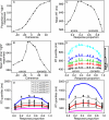
A-D. Plots of data from a motion discrimination experiment, Experiment 1 [7]. A Response proportion plotted against motion coherence. B Mean RT plotted against motion coherence. C Mean RT plotted against response proportion. D RT quantiles plotted against response proportion for data (digits) and model predictions (o's and lines). The quantiles used were the .1, .3, .5, .7, and .9 quantiles and these represent, respectively, the fastest 10% of responses, the fastest 30%, the median RT, the slowest 30%, and the slowest 10%. The quantiles are stacked vertically and the small inset to the right shows equal-area rectangles drawn between quantiles to illustrate what RT distributions derived from the quantiles would look like. E-F. Fits to a data set that has large differences in the leading edge of the RT distribution, changes too large for a diffusion model with only drift rate changing over conditions to fit (from Experiment 1, [38]). E Data and predictions for fits to RT distribution quantiles. The .1 quantile (magenta) and median (red) miss the data. F Data and predictions for RT quantiles for fits to accuracy and median RT. The median (red) fits well, but the other quantiles miss badly.

Figure 4

Modeling the response signal procedure and collapsing boundaries.

Figure 5. Brief stimulus presentation. Does the decision process track stimulus information?

A shows drift rate as a function of time for the model in which drift tracks the stimulus (here turning on at zero and off at 80 ms). B shows the mean and plus and minus 1 standard deviation average paths from simulations (using the random walk method, [116]). The red arrow is the point that drift rate turns off and the horizontal red lines are the decision boundaries. C shows RT distributions for correct responses for the simulations with the red circles showing the .1, .3, .5, .7, and .9 quantile RTs. D shows RT distributions for error responses for the simulations with the blue circles showing the .1, .3, .5, .7, and .9 quantile RTs (the red circles are the quantiles for the correct responses from C).

References

1. Ratcliff R, Smith PL. A comparison of sequential sampling models for two-choice reaction time. Psychol. Rev. 2004;111:333–367. - PMC - PubMed
1. Ratcliff R. A theory of memory retrieval. Psychol. Rev. 1978;85:59–108.
1. Ratcliff R. A theory of order relations in perceptual matching. Psychol. Rev. 1981;88:552–572.
1. Ratcliff R, Rouder JN. Modeling response times for two-choice decisions. Psychol. Sci. 1998;9:347–356.
1. Ratcliff R, et al. Connectionist and diffusion models of reaction time. Psychol. Rev. 1999;106:261–300. - PubMed
Publication types
LinkOut - more resources