ConceFT: concentration of frequency and time via a multitapered synchrosqueezed transform

Abstract

A new method is proposed to determine the time-frequency content of time-dependent signals consisting of multiple oscillatory components, with time-varying amplitudes and instantaneous frequencies. Numerical experiments as well as a theoretical analysis are presented to assess its effectiveness.

Keywords: ConceFT; instantaneous frequency; multitaper; reassignment method; synchrosqueezing transform.

Figure 1.

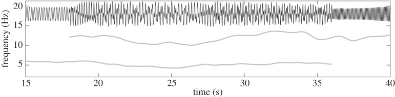
The signal s (top, in black) and the corresponding instantaneous frequencies (below, in grey) of the two components, restricted to the time interval [15,40].

Figure 2.

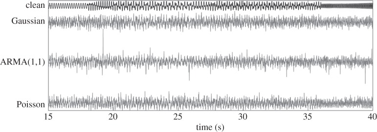
The restrictions to [15,40] of the clean signal s (top) and of the noisy signal Y =s+σξ, where the added noise is Gaussian, ARMA(1,1), or Poisson noise (below, in order); in each case σ is picked so that the noisy signal has 0 dB SNR. All signals are plotted at the same scale.

Figure 3.

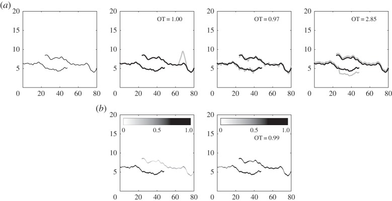
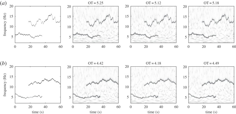
(a) Left: the TF localization of the itvPS of a two-component simulated signal s_a (not showing the amplitude modulation (AM)). Other itvPS shown in the top row are for signals s_b, s_c and s_d that have a fairly small different OT distance with respect to s_a; the two components have the same time-dependent amplitudes as for s_a, but the instantaneous frequency curves have been moved (in order from left to right) by a narrow bump (left), a random dither (middle) and a shift (right). (b) Illustration of amplitude change. Left: the original itvPS of s_a with the AM values indicated by grey scale level; right: an itvPS example with the same IF but different AM. In all panels, the horizontal axis is time and the vertical axis is frequency. The image for each ‘deformed’ itvPS indicates its OT distance to the original itvPS (shown in the leftmost image on each row).

Figure 4.

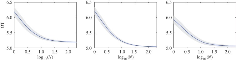
The OT distance as a function of the number N of random projections. The shaded band indicates the standard deviation of the OT distance at the corresponding number of random projections. From left to right, the noise types are Gaussian, ARMA(1,1) and Poisson, respectively. For all three experiments, β=30, γ=9 and the first two Morse wavelets are used. (Online version in colour.)

Figure 5.

(a) Results for the signal s; (b) results for a new example s*. Left to right: ideal time-varying TF power spectrum (itvPS) for the clean signal, followed by results of ConceFT with Morse wavelets after (in order) Gaussian, ARMA(1,1) or Poisson noise was added, with SNR of 0 dB. Clearly, even for an SNR as low as 0 dB, the results approximate the truth with high precision. For each of the tvPS panels, the header gives the OT distance to the corresponding itvPS.

Figure 6.

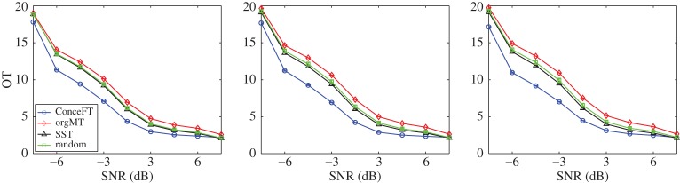
OT distance of ConceFT tvPS results against SNR of the signal s*(t), and comparison with standard SST and standard multitaper SST (see text). Noise type (left to right): Gaussian, ARMA(1,1) and Poisson. The standard deviation is smaller, at the scale of this figure, than the height of the markers, and has not been plotted. (Online version in colour.)

Figure 7.

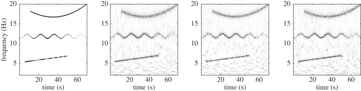
Results for the three-component deterministic signal s°. Left: ideal time-varying TF power spectrum (itvPS) for the clean signal, followed by results of ConceFT with Morse wavelets after (in order) Gaussian, ARMA(1,1) or Poisson noise was added, with SNR of 0 dB.