Four-dimensional maps of the human somatosensory system

Abstract

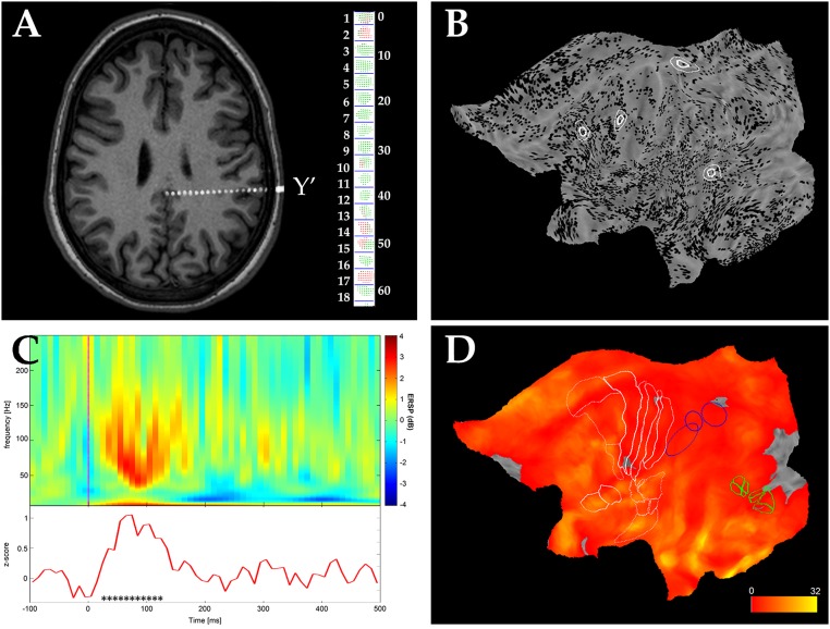
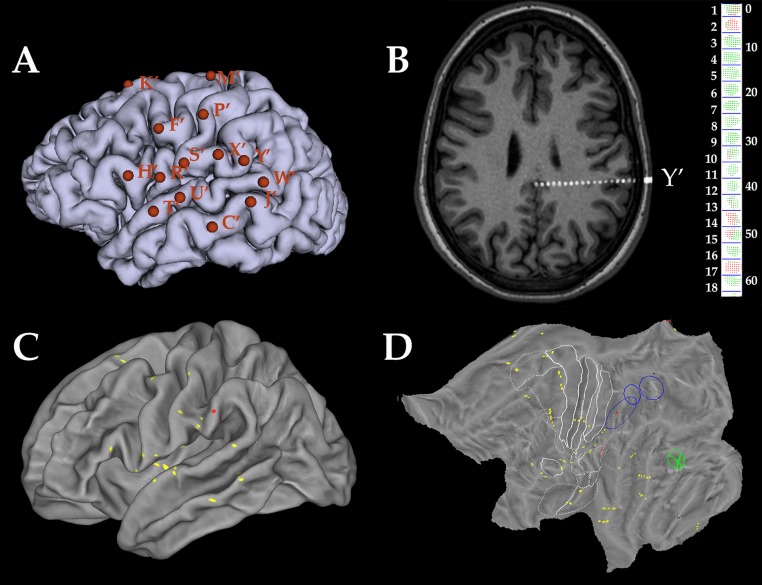
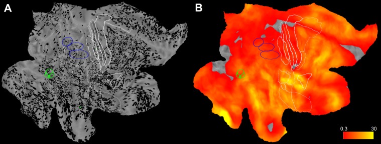
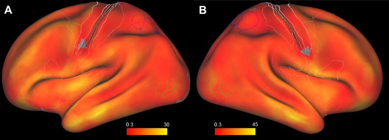
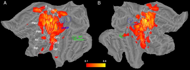
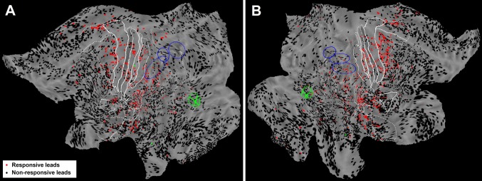
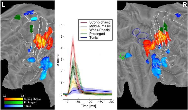
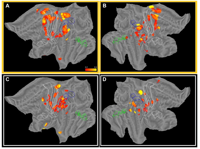
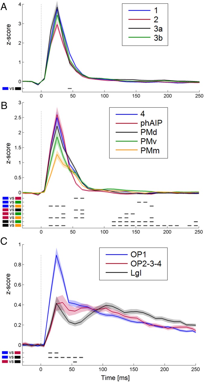
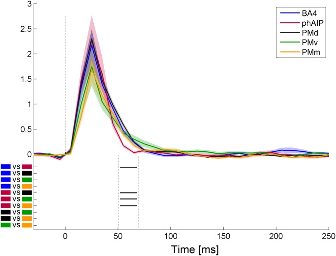
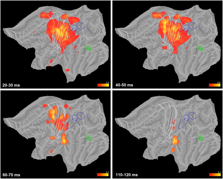
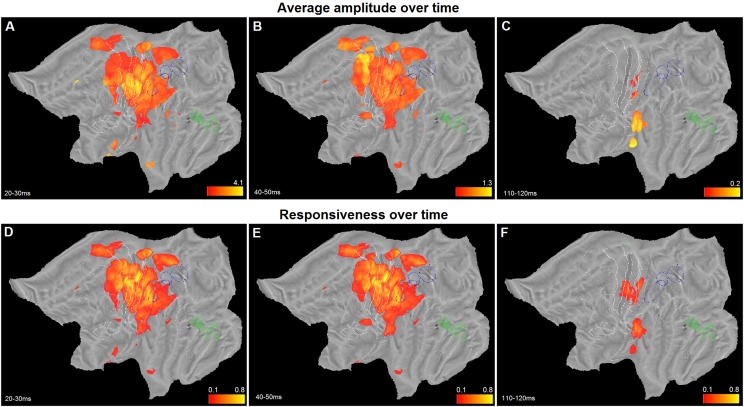
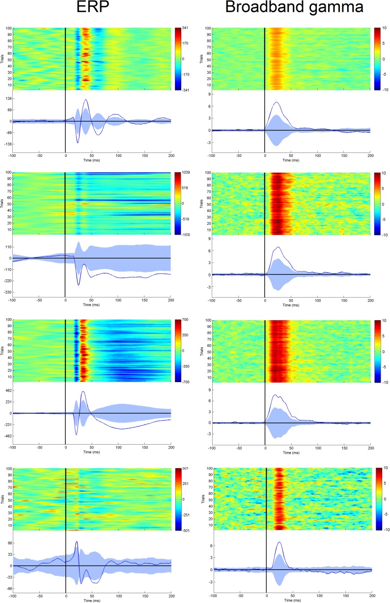
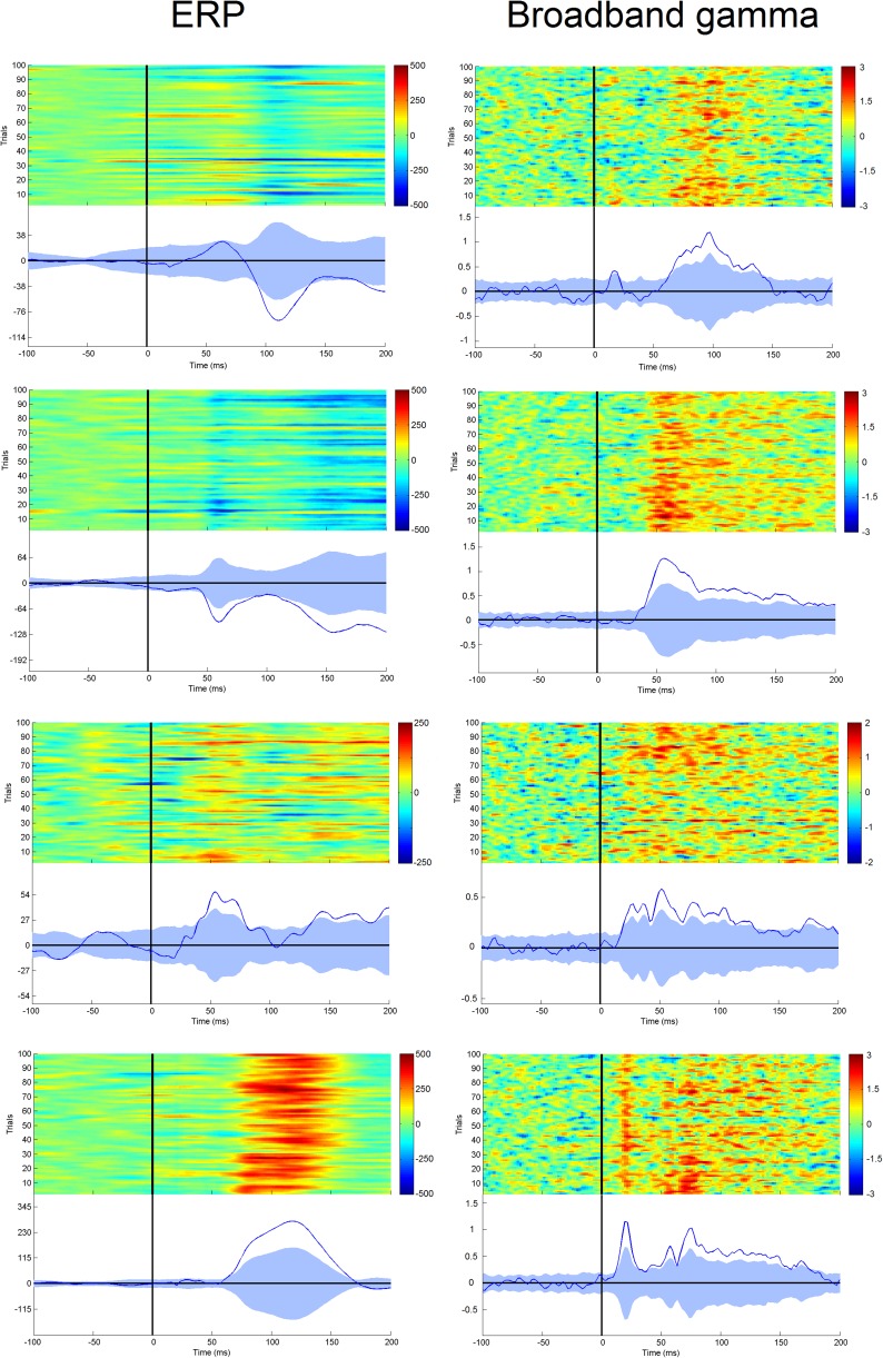
A fine-grained description of the spatiotemporal dynamics of human brain activity is a major goal of neuroscientific research. Limitations in spatial and temporal resolution of available noninvasive recording and imaging techniques have hindered so far the acquisition of precise, comprehensive four-dimensional maps of human neural activity. The present study combines anatomical and functional data from intracerebral recordings of nearly 100 patients, to generate highly resolved four-dimensional maps of human cortical processing of nonpainful somatosensory stimuli. These maps indicate that the human somatosensory system devoted to the hand encompasses a widespread network covering more than 10% of the cortical surface of both hemispheres. This network includes phasic components, centered on primary somatosensory cortex and neighboring motor, premotor, and inferior parietal regions, and tonic components, centered on opercular and insular areas, and involving human parietal rostroventral area and ventral medial-superior-temporal area. The technique described opens new avenues for investigating the neural basis of all levels of cortical processing in humans.

Keywords: cerebral cortex; intracranial recordings; median nerve; stereo-EEG; temporal dynamics.

Fig. 1.

Anatomical and functional data analysis. (A) Axial MR slice of a patient, after the coregistration with the postimplantation CT, on which the entire Y′ electrode implanted in the left hemisphere is visible. The reconstruction of the Y′ electrode is shown on the right side, with the leads numbered 1–18 from the tip, for a total distance of 50 mm. Leads are represented by sets of voxels, colored red if located in cortical gray matter and green otherwise. (B) Midthickness surface of the fs_LR brain template with all leads located in gray matter of the left hemisphere (from 49 patients) indicated as black dots. For four nodes, circles with 0.5 cm (thick line) and 1 cm (thin line) of radius represent the masks. (C, Upper) Average time frequency plot (100 trials) in response to median nerve stimulation in one lead of one patient. (C, Lower) Time course of the average gamma power (50–150 Hz) for the same channel, reported as z scores based on the prestimulus interval. Black asterisks indicate time bins with gamma power significantly exceeding baseline (P < 0.001). (D) Sampling density of the left hemisphere computed from data in B. The color scale is expressed in the number of recording leads per cm². Cytoarchitectonic areas (1–4, 6, OP1–4, and 44) and anatomically defined areas (long and short gyri of insula) are indicated by white lines, and functionally defined regions are indicated in blue [confidence ellipses of phAIP, DIPSA, and DIPSM from Jastorff et al. (78)] or green [MT cluster from Abdollahi et al. (72)].

Fig. S1.

Single-patient anatomical data processing. (A) Lateral view of the left hemisphere of a patient with the entry points of 14 implanted electrodes marked by orange letters (with asterisks to indicate left side). (B) Axial MR slice from the same patient, after the coregistration with the cone-beam CT, on which the entire Y′ electrode is visible. The reconstruction of the Y′ electrode is shown on the right side, with the leads numbered from the tip of the electrode. Leads are represented by sets of voxels colored in red if located in gray matter and green otherwise. (C) Midthickness surface of the same patient warped to the fs_LR brain template with all leads exploring gray matter projected onto the surface and indicated in yellow. The leads of electrode Y′ are indicated in red. (D) Same data as C shown on a flat map of the left hemisphere. Note that whereas in C, only the three outermost leads of electrode Y′ are visible, flat map visualizes all leads located in cortical gray matter.

Fig. S2.

Sampling in right hemisphere. (A) Midthickness surface of the fs_LR brain template with all leads located in gray matter of the right hemisphere (from 58 patients) indicated as black dots. Anatomical and functional borders are defined as in Fig. 2. (B) Sampling density of the right hemisphere computed from data in A.

Fig. S3.

Inflated view of sampling density of the left (A) and right (B) hemispheres.

Fig. 2.

Overall responsiveness maps. Overall responsiveness (responsive leads as a percentage of total explored leads per disk) maps for the left (A) and right (B) hemispheres. Only surface nodes with values exceeding 10% were shown. The same conventions as in Fig. 1 are used.

Fig. S4.

Responsive leads. (A and B) Midthickness surface of the fs_LR brain template with all leads located in gray matter of left (49 patients) (A) and right (58 patients) (B) hemisphere. Red dots indicate responsive leads, and black dots nonresponsive ones. The same conventions as in Fig. 1 are used.

Fig. 3.

Clustering of time courses. (Center) Time courses (centroid ± SD) of the five clusters, as indicated (Inset). (Left and Right) Relative responsiveness (leads belonging to one cluster as a percentage of total number of responsive leads per disk) maps of left (L) and right (R) hemispheres (middle portion) for strong-phasic (yellow red), delayed-phasic (green), and tonic (blue) clusters. Only nodes with values exceeding 20% are shown. The same conventions as in Fig. 1 are used.

Fig. S5.

Relative responsiveness maps of middle (A and B) and weak-phasic (C and D) clusters on flat maps of the left (A and C) and right (B and D) hemispheres. Color coding is as in Fig. 3. The yellow frame indicates weak-phasic, and the black frame indicates middle-phasic.

Fig. 4.

ROI analysis. Average (±SE) time course of leads in somatosensory areas (A), motor regions (B), and opercular/insular areas (C). Areas are listed (Insets). Black marks under the curves indicate significant post hoc comparisons (P < 0.002). Number of responsive leads for each graph: 34 in area 1, 54 in area 2, 21 in area 3a, 50 in area 3b (A); 68 in area 4, 157 in PMd, 45 in medial premotor areas, 42 in PMv, and 28 in phAIP (B); and 133 in OP1, 54 in other OPs, and 38 in LgI (C).

Fig. S6.

Subthreshold results. Average (±SE) time course of leads in motor areas (Inset) following submotor threshold stimulation of median nerve. Black marks under the curves indicate significant post hoc comparisons (P < 0.02) for the average gamma power between 50 and 70 ms.

Fig. 5.

Weighted amplitude maps over time. Four weighted amplitude maps of the left hemisphere at time bins indicated. The color range is dynamically adjusted from frame to frame. Note how the activity peaks in primary sensory areas in first frame, spreads to dorsal premotor area (second frame), remains active longer (third frame), whereas residual activity after 100 ms is recorded mostly from parietal operculum (OP1) and long gyri of insula (last frame). The same conventions as in Fig. 1 are used.

Fig. S7.

Average amplitude and responsiveness over time. Three average amplitude (A–C) and responsiveness (D–F) maps of the left hemisphere at time bins indicated. The color range for average amplitude is dynamically adjusted from frame to frame. The same conventions as in Fig. 1 are used.

Fig. S8.

Comparison of intracranial ERP (left column) and broadband gamma (right column). Responses in four leads (four different patients) recording from area 3b. The color scale indicates voltage and z scores, respectively.

Fig. S9.

Comparison of intracranial ERP (left column) and broadband gamma (right column). Responses in four leads (four different patients) recording from area OP1. The color scale indicates voltage and z scores, respectively. Note that two of the four leads (first and last rows) exhibit a mixed pattern, composed of a phasic activity followed by a tonic one. Although this pattern is poorly visible in the ERP response, it appears evidently in the gamma band time course.

References

1. Van Essen DC. Cartography and connectomes. Neuron. 2013;80(3):775–790. - PMC - PubMed
1. Kopell NJ, Gritton HJ, Whittington MA, Kramer MA. Beyond the connectome: The dynome. Neuron. 2014;83(6):1319–1328. - PMC - PubMed
1. Hari R, Parkkonen L. The brain timewise: How timing shapes and supports brain function. Philos Trans R Soc Lond B Biol Sci. 2015;370(1668):pii: 20140170. - PMC - PubMed
1. Burle B, et al. Spatial and temporal resolutions of EEG: Is it really black and white? A scalp current density view. Int J Psychophysiol. 2015;97(3):210–220. - PMC - PubMed
1. Debener S, Ullsperger M, Siegel M, Engel AK. Single-trial EEG-fMRI reveals the dynamics of cognitive function. Trends Cogn Sci. 2006;10(12):558–563. - PubMed
Publication types