Low-dimensional dynamics of structured random networks

Abstract

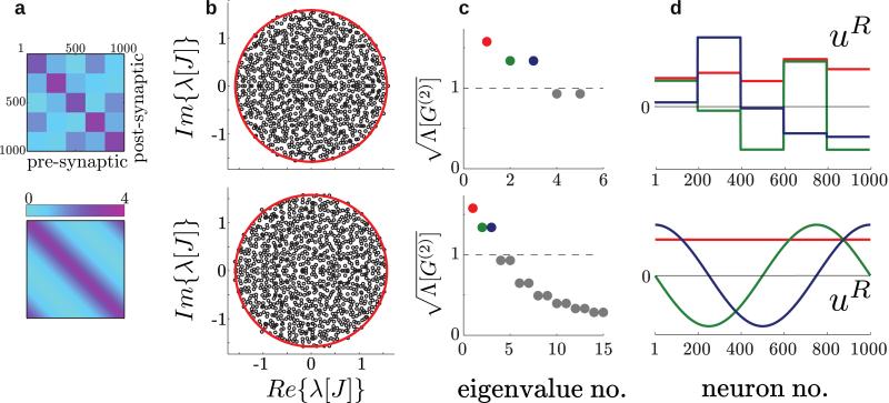
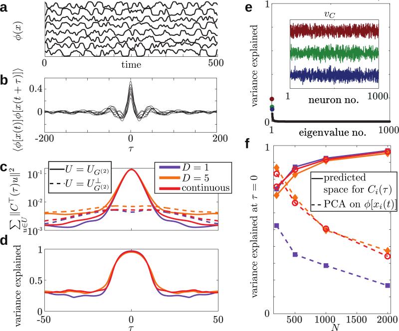
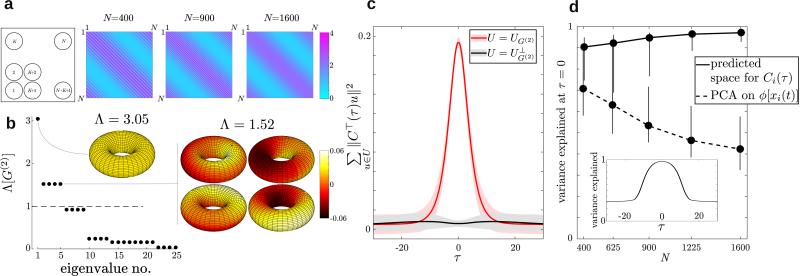
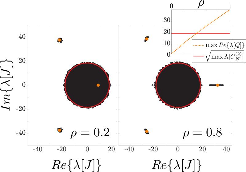
Using a generalized random recurrent neural network model, and by extending our recently developed mean-field approach [J. Aljadeff, M. Stern, and T. Sharpee, Phys. Rev. Lett. 114, 088101 (2015)], we study the relationship between the network connectivity structure and its low-dimensional dynamics. Each connection in the network is a random number with mean 0 and variance that depends on pre- and postsynaptic neurons through a sufficiently smooth function g of their identities. We find that these networks undergo a phase transition from a silent to a chaotic state at a critical point we derive as a function of g. Above the critical point, although unit activation levels are chaotic, their autocorrelation functions are restricted to a low-dimensional subspace. This provides a direct link between the network's structure and some of its functional characteristics. We discuss example applications of the general results to neuroscience where we derive the support of the spectrum of connectivity matrices with heterogeneous and possibly correlated degree distributions, and to ecology where we study the stability of the cascade model for food web structure.

FIG. 1

Eigenspaces of two example networks – one with block structured connectivity (top) and another with continuous gain modulation (bottom). (a) The synaptic gain matrix g_ij. (b) The spectrum of the random connectivity matrix J in the complex plane. The spectrum is supported by a disk with radius $r=\sqrt{{\Lambda }_1}$ indicated in red. (c) The square root of the largest eigenvalues of $G_N^{\left(2\right)}$. When these are greater than 1, the corresponding eigenvectors [shown in (d)] are active autocorrelation modes. For the continuous function we chose the circulant parametrization (see Sec. IV A) with g₀ = 0.3, g₁ = 3.0 and γ = 2.0. For the block structured connectivity, g was chosen such that the first five eigenvalues match exactly to those of the continuous network.

FIG. 2

Low-dimensional structure of network dynamics. Traces of the firing rates ϕ[x_i(t)] (a) and autocorrelations C_i(τ) (b) of eight example neurons chosen at random from the network with continuous gain modulation (shown in the bottom row of Fig. 1). (c) The sum of squared projections of the vector C_i(τ) on the vectors spanning U_G⁽²⁾ (the active modes, solid lines) or $U_{G^{\left(2\right)}}^{\perp }$ (the inactive modes, dashed lines). The dimension of the subspace U_G⁽²⁾ is K★ = 1 for the network with g = const and K★ = 3 for the block and continuous cases (orange and red, respectively), much smaller than N – K★ ≈ N, orthogonal the dimension of the complement space $U_{G^{\left(2\right)}}^{\perp }$. (d) Our analytically derived subspace accounts for almost 100 percent of the variance in the autocorrelation vector for $\mid \tau \mid \lesssim 10$ (in units of the synaptic time constant). (e) Reducing the dimensionality of the dynamics via principal component analysis on ϕ(x) leads to vectors (inset) that account for a much smaller portion of the variance (when using same dimension K★ for the subspace), and lack structure that could be related to the connectivity. (f) Summary data from 50 simulated networks per parameter set (N, structure type) at τ = 0. As N grows the leak into $U_{G^{\left(2\right)}}^{\perp }$ diminishes if one reduces the space of the C_i(τ) data while the fraction of variance explained becomes smaller when using PCA on the ϕ[x_i(t)] data, a signature of the extensiveness of the dimension of the chaotic attractor.

FIG. 3

Results for a toroidal network. (a) A grid strategy with $K=\sqrt{N}$ for tiling the [0, 1] × [0, 1] torus with N neurons (left) and the resulting deterministic gain matrix with elements g_ij for three values of N as defined in Eq. (35) (right). Unlike the ring network, here g depends on N, and its derivative is unbounded so as N increases the gain function “folds.” The parameters of the connectivity matrix are g₀ = 0.7, g₁ = 0.8. (b) The 25 nonzero eigenvalues of $G_N^{\left(2\right)}$ for N = 1600 and the eigenvectors corresponding to eigenvalues that are greater than 1 plotted on a torus with coordinates $({\theta }_i^1,{\theta }_i^2)$. (c) The sum of squared projections of the vector C_i(τ) on the vectors spanning U_G(2) (the active modes, red line) or $U_{G^{\left(2\right)}}^{\perp }$ (the inactive modes, black line). Shades indicate the standard deviation computed from 50 realizations. (d) Comparison of the variance explained at τ = 0 by our predicted subspace (solid line) and by performing PCA on ϕ(x) (dashed line). Error bars represent 95% confidence intervals. Inset: the subspace we derived accounts for a large portion of the variance for time lags $\mid \tau \mid \lesssim 10$ (in units of the synaptic time constant).

FIG. 4

Spectrum of connectivity matrices with heterogeneous, correlated joint degree distribution. The network parameters were chosen to be κ = 0.7, θ = 28.57, N_E = 1000, N_I = 250, p₀ = 0.05, W₀ = 5, where κ and θ are the form and scale parameters respectively of the distribution from which the in- and out-degree sequences are randomly drawn. The average correlation ρ between the in- and out-degree sequences was varied between 0 and 1. For the values ρ = 0.2 (left) and ρ = 0.8 (right) we drew 25 degree sequences and based on them drew the connectivity matrix according to the prescription outlined in Sec. V. The eigenvalues of each matrix were computed numerically and are shown in black. For each value of ρ we computed the average functions $\langle \mathcal{T}\rangle$, $\langle \mathcal{S}\rangle$ etc., and the roots of the characteristic polynomials $\mathcal{A}\left(\Lambda \right)$ and $\mathcal{B}\left(\lambda \right)$ (see Appendixes B and C for derivation). The predictions for the support of the bulk (solid red line) and the outliers (orange points and dotted line) are in agreement with the numerical calculation. Inset: as a function of ρ, there is a positive outlier that exits the disk to the right.

References

1. Kleinfeld D, Bharioke A, Blinder P, Bock DD, Briggman KL, Chklovskii DB, Denk W, Helmstaedter M, Kaufhold JP, Lee W-CA, Meyer HS, Micheva KD, Oberlaender M, Prohaska S, Reid RC, Smith SJ, Takemura S, Tsai PS, Sakmann B. The Journal of Neuroscience. 2011;31:16125. - PMC - PubMed
1. Ko H, Hofer SB, Pichler B, Buchanan KA, Sjöström PJ, Mrsic-Flogel TD. Nature. 2011;473:87. - PMC - PubMed
1. Karlebach G, Shamir R. Nature Reviews Molecular Cell Biology. 2008;9:770. - PubMed
1. Chung K, Deisseroth K. Nature Methods. 2013;10:508. - PubMed
1. Song S, Sjöström PJ, Reigl M, Nelson S, Chklovskii DB. PLoS Biology. 2005;3:e68. - PMC - PubMed
Publication types
LinkOut - more resources