Integrative NMR for biomolecular research

Abstract

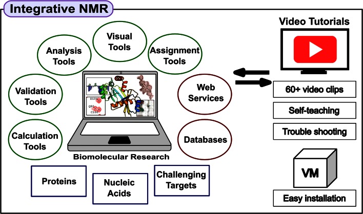
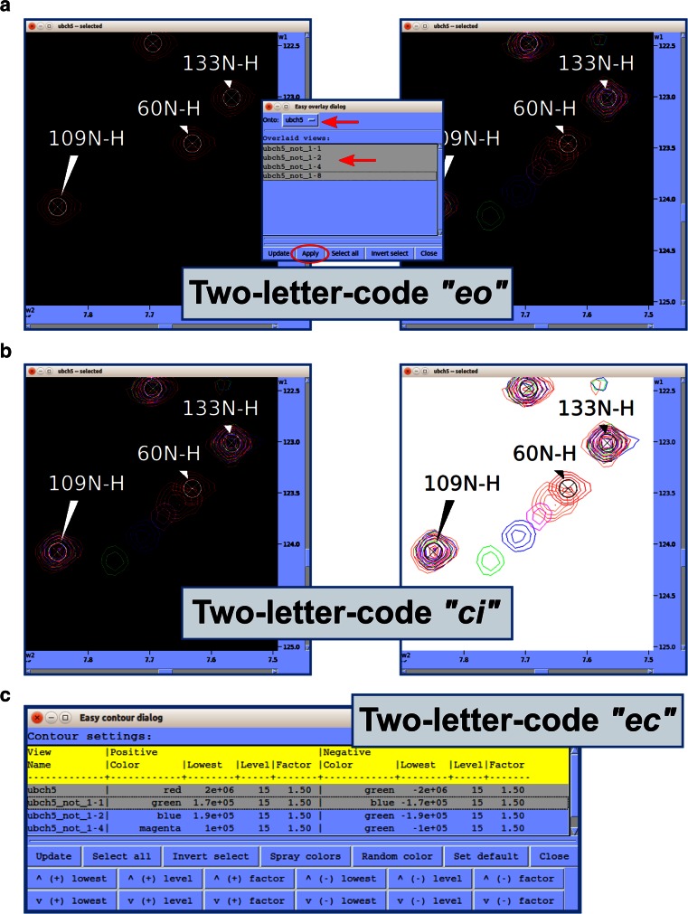
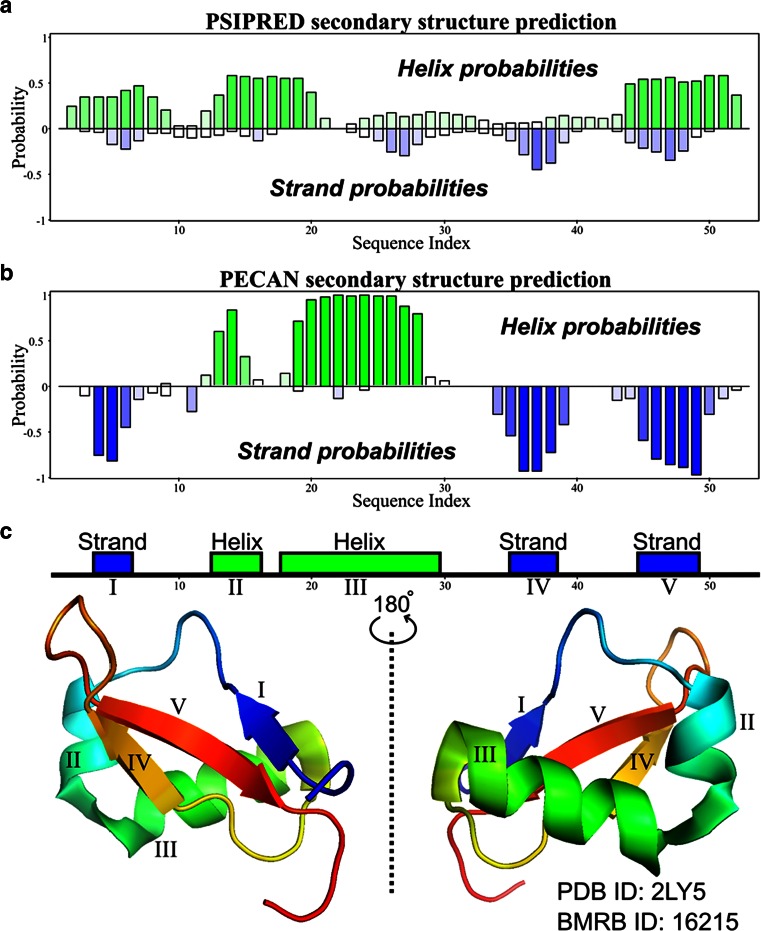
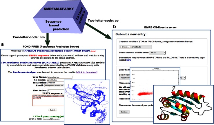
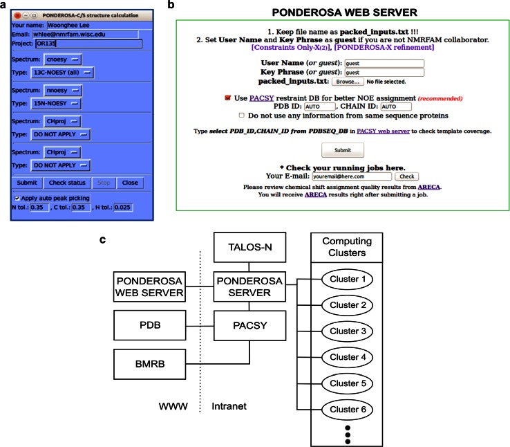
NMR spectroscopy is a powerful technique for determining structural and functional features of biomolecules in physiological solution as well as for observing their intermolecular interactions in real-time. However, complex steps associated with its practice have made the approach daunting for non-specialists. We introduce an NMR platform that makes biomolecular NMR spectroscopy much more accessible by integrating tools, databases, web services, and video tutorials that can be launched by simple installation of NMRFAM software packages or using a cross-platform virtual machine that can be run on any standard laptop or desktop computer. The software package can be downloaded freely from the NMRFAM software download page ( http://pine.nmrfam.wisc.edu/download_packages.html ), and detailed instructions are available from the Integrative NMR Video Tutorial page ( http://pine.nmrfam.wisc.edu/integrative.html ).

Keywords: Automated spectral analysis; Automated structure determination and validation; Chemical shift assignment and validation; Peak identification; Restraint visualization and validation; Visualization of spectra, assignments, and structures.

Fig. 1

The Integrative NMR method for conducting biomolecular research. This integrated set of software packages, which can be installed on a laptop or desktop computer—optionally as part of a virtual machine, cover a wide range of data analysis and visualization steps in the workflows of biomolecular NMR research. The software tools interoperate seamlessly with external servers and databases. Video tutorials cover all operations

Fig. 2

Recommended semi-automated peak identification method in NMRFAM-SPARKY. a Use APES (two-letter-code ae) or restricted peak picking (two-letter-code kr) for automated peak identification. b Use alternative peak list window (two-letter-code LT) to sort peaks by intensities. c Delete weak noise peaks from spectrum view. d Use strip plot (two-letter-code sp) to delete any remaining false-positive peaks and add missing peaks

Fig. 3

Predict-and-confirm method for fast semi-automated chemical shift assignment. a Efficient method for assigning a C(CO)NH spectrum. In the Transfer and simulate assignment window (two-letter-code: ta), set Spectrum and Type; then click the Simulate button to annotate predicted assignments on the experimental spectrum (yellow ‘X’s). Drag each yellow X onto the nearest peak in the spectrum, and type “cu” to confirm the assignment. The yellow ‘X’s are now centered on the position of the experimental peak. b Illustration of how Predict-and-confirm can be used to import assignments from a BMRB entry. The BMRB assignments are displayed over the spectrum, and the user can then adjust and confirm them

Fig. 4

Dummy Graph is molecular structure visualization tool that shows the atoms in a three-residue stretch and indicates which atoms have been assigned. Also shown is the average chemical shift and standard deviation (in ppm) from the positions of all peaks in the different spectra supporting a given assignment. An atom can be selected by clicking; this turns its background pink as shown for T7CA. The panel at the bottom shows assignments (in the Label List) related to the selected atom from the spectrum selected in the Spectra List. a A thick line around an atom and chemical shift indicates that the atom is already assigned. Otherwise, a thin line around an atom indicates that it is not yet assigned. b Large chemical shift deviations are written in purple to alert the user to the possibility of an erroneous assignment

Fig. 5

Tools developed for assisting chemical shift assignment of nucleic acids. a NMRFAM-SPARKY supports covariance ellipses for RNA ¹H and ¹³C chemical shifts first introduced in the CHESS2FLYA program. Statistical ellipses is a tool in NMRFAM-SPARKY (two-letter-code SE) that overlays color-coded ellipses on the spectra to outline the range of chemical shifts expected for different RNA bases. The peaks underlined in cyan are near the center of the cyan ellipse, which corresponds to Uracil. b Dummy Graph for Nucleic Acids (two-letter-code DG) is a tool for visualizing atoms of DNA or RNA residues; base atoms of are shown at the top and those of the sugar and phosphate are shown at the bottom. The panel below shows assignments related to the selected atom shown in pink (U4H6) from the selected spectrum

Fig. 6

NDPPlot is a tool fully integrated into NMRFAM-SPARKY for visualizing spectral changes. a Perturbation plot (two-letter-code np). The arrows point to the change in the chemical shift of residue 96. The contour plot overlays (two-letter-code ol or eo) two selected ¹H–¹⁵N HSQC spectra: one recorded with (green contour) and one without (red contour) added substrate. The displacement of the signal assigned to residue 96 is highlighted within the circle. NDPPlot generates the bar chart shown to plot the chemical shift differences between two spectra along the sequence; this is achieved by choosing the two spectra and the observable to be compared (in this case, the chemical shift of amide protons) in the Perturbation plot window and by clicking Plot. b Titration Plot (two-letter-code ni) visualizes chemical shift changes from a titration experiment. Results are plotted by the NDPPlot program. This example shows how the ¹H NMR chemical shift of residue 96 from the ¹H-¹⁵N HSQC spectra changes upon the addition of a substrate. The spectrum shows the overlap (two-letter-code ol) of spectra without and with four increasing levels of added substrate. Contour colors are set by the two-letter-code ct (with 0 for red, 1/8 for tomato, 1/4 for magenta, 1/2 for blue, 1 for green). In the Titration Plot window, by choosing the spectra and the observable to be compared (in this case, the ¹H chemical shift of H96) and clicking the Plot button, NDPPlot graphs ¹H NMR chemical shift of H96 as a function of the molar ratio. c The Peak Height Analysis tool (two-letter-code rh) can be used to analyze results from relaxation experiments or any other peak intensity related experiments. After choosing a series of assigned spectra with different time/condition parameters, clicking the Plot T-decay button can be used to visualize the relaxation time constant as a function of residue number or by choosing a single residue, the decay in its peak intensity over time/condition. Alternatively, per residue and per spectrum intensity analysis options are available for observing overall differences between residues or spectra

Fig. 6

NDPPlot is a tool fully integrated into NMRFAM-SPARKY for visualizing spectral changes. a Perturbation plot (two-letter-code np). The arrows point to the change in the chemical shift of residue 96. The contour plot overlays (two-letter-code ol or eo) two selected ¹H–¹⁵N HSQC spectra: one recorded with (green contour) and one without (red contour) added substrate. The displacement of the signal assigned to residue 96 is highlighted within the circle. NDPPlot generates the bar chart shown to plot the chemical shift differences between two spectra along the sequence; this is achieved by choosing the two spectra and the observable to be compared (in this case, the chemical shift of amide protons) in the Perturbation plot window and by clicking Plot. b Titration Plot (two-letter-code ni) visualizes chemical shift changes from a titration experiment. Results are plotted by the NDPPlot program. This example shows how the ¹H NMR chemical shift of residue 96 from the ¹H-¹⁵N HSQC spectra changes upon the addition of a substrate. The spectrum shows the overlap (two-letter-code ol) of spectra without and with four increasing levels of added substrate. Contour colors are set by the two-letter-code ct (with 0 for red, 1/8 for tomato, 1/4 for magenta, 1/2 for blue, 1 for green). In the Titration Plot window, by choosing the spectra and the observable to be compared (in this case, the ¹H chemical shift of H96) and clicking the Plot button, NDPPlot graphs ¹H NMR chemical shift of H96 as a function of the molar ratio. c The Peak Height Analysis tool (two-letter-code rh) can be used to analyze results from relaxation experiments or any other peak intensity related experiments. After choosing a series of assigned spectra with different time/condition parameters, clicking the Plot T-decay button can be used to visualize the relaxation time constant as a function of residue number or by choosing a single residue, the decay in its peak intensity over time/condition. Alternatively, per residue and per spectrum intensity analysis options are available for observing overall differences between residues or spectra

Fig. 6

NDPPlot is a tool fully integrated into NMRFAM-SPARKY for visualizing spectral changes. a Perturbation plot (two-letter-code np). The arrows point to the change in the chemical shift of residue 96. The contour plot overlays (two-letter-code ol or eo) two selected ¹H–¹⁵N HSQC spectra: one recorded with (green contour) and one without (red contour) added substrate. The displacement of the signal assigned to residue 96 is highlighted within the circle. NDPPlot generates the bar chart shown to plot the chemical shift differences between two spectra along the sequence; this is achieved by choosing the two spectra and the observable to be compared (in this case, the chemical shift of amide protons) in the Perturbation plot window and by clicking Plot. b Titration Plot (two-letter-code ni) visualizes chemical shift changes from a titration experiment. Results are plotted by the NDPPlot program. This example shows how the ¹H NMR chemical shift of residue 96 from the ¹H-¹⁵N HSQC spectra changes upon the addition of a substrate. The spectrum shows the overlap (two-letter-code ol) of spectra without and with four increasing levels of added substrate. Contour colors are set by the two-letter-code ct (with 0 for red, 1/8 for tomato, 1/4 for magenta, 1/2 for blue, 1 for green). In the Titration Plot window, by choosing the spectra and the observable to be compared (in this case, the ¹H chemical shift of H96) and clicking the Plot button, NDPPlot graphs ¹H NMR chemical shift of H96 as a function of the molar ratio. c The Peak Height Analysis tool (two-letter-code rh) can be used to analyze results from relaxation experiments or any other peak intensity related experiments. After choosing a series of assigned spectra with different time/condition parameters, clicking the Plot T-decay button can be used to visualize the relaxation time constant as a function of residue number or by choosing a single residue, the decay in its peak intensity over time/condition. Alternatively, per residue and per spectrum intensity analysis options are available for observing overall differences between residues or spectra

Fig. 7

Useful tools for spectral series analysis. a Easy overlay dialog. We developed much simpler tool for spectral overlay than traditional “ol” tool particularly for many spectra. It is activated by two-letter-code “eo”. Simply, user can choose a spectrum “onto” and select spectra to “overlay” by mouse dragging and clicking with Ctrl and Shift keys. When most of all spectra in the project need to be overlaid, user can simply click Select all button and exclude spectra by Ctrl key and mouse clicks. b Change inverse background. We understood the visual limitation of black background color for spectral series analysis if user needs to color spectra differently. Thus, we developed two-letter-code “ci” to change background color from black to white and from white to black. The background color can be set differently and if ornament color is black and white, they are automatically changed to the other color, and so markers such as crosshair are. c Easy contour dialog. This tool is activated by two-letter-code “ec”. It can be used to adjust contour color, level and threshold of multiple spectra all at once

Fig. 8

Sequence-based and chemical shift-based predictions from NMRFAM-SPARKY of the secondary structure of the protein brazzein (PDB ID: 2LY5, BMRB ID: 16215). The illustration was made by NDPPlot. a Sequence-based prediction by PSIPRED (two-letter-code PP) could not predict secondary structures correctly and the probabilities are not confident. b Chemical shift-based prediction by PECAN (two-letter-code n6). c Secondary structures from PDB deposited structure. The PECAN prediction matched perfectly with the secondary structural elements determined from the structure

Fig. 9

Three-dimensional structures can be predicted by sequence-based method and chemical shift-based methods in NMRFAM-SPARKY. a POND-PRED (two-letter-code nm) is a webserver offered by NMRFAM for predicting protein 3D structures from amino acid sequences. b CS-Rosetta is a chemical shift-based 3D structure prediction program; it is accessibly from NMRFAM-SPARKY (two-letter-code ce) on a web server hosted by BMRB

Fig. 10

NMR-based 3D protein structure calculation. a Calculation 3D structure by PONDEROSA-C/S (two-letter-code c3) offers direct job submission from NMRFAM-SPARKY to the Ponderosa Web Server. It supports fully automated mode with and without automated NOESY peak picking and semi-automated mode with partially or fully assigned NOESY data. b Ponderosa Web Server is a freely available web resource that transmits the structure calculation command to the Ponderosa Server running at NMRFAM. c Diagram showing the integrated architecture of Ponderosa Web Server and Ponderosa Server at NMRFAM

Fig. 11

Ponderosa Client supports several formats and settings for structure calculation. a Ponderosa Client accepts several types of input including NOE (raw spectra: .ucsf, .pipe; peak list: .peaks, .list, .xpk, 3rrr), RDC (.rdc), and SAXS (.dat) for Xplor-NIH based structural calculations. b The optimized noise threshold for NOESY peak picking is determined automatically by Intensity Plot, which ranks the intensities of NOE peaks and uses an r ⁻⁶ (r: distance between two protons) approach to estimate the intensity corresponding to the 5.5 Å cutoff (blue robust range, black mixture of real peaks and noise, red noise range). c Alternatively, the user can employ the Visual Select tool to determine the noise level. This tool randomly selects a position where the chemical shift assignments suggest that a peak should be found, and the user decides whether the signal is a real peak or noise. d The Visual Select tool is integrated with NMRFAM-SPARKY for better decision making. Clicking the peak position in the Visual Select tool enables the user to navigate (two-letter-code up) to the position of the peak in a spectrum displayed by NMRFAM-SPARKY

Fig. 12

Ponderosa Analyzer provides tools for validating assignments, constraints and structures that are integrated with Enhanced PyMOL and NMRFAM-SPARKY. a Distance Constraint Validator is a tool for analyzing distance information extracted from NOESY data. b 3D illustration of the constraint selected (Enhanced PyMOL command @p). c NOESY spectrum highlighting the experimental evidence for the selected constraint (NMRFAM-SPARKY two-letter-code up). The user can manually adjust or exclude the examined constraint for the next run by means of the Constraint Control buttons in the Distance Constraint Validator

Fig. 13

H-bond manager is a Ponderosa Analyzer tool that provides an easy way to add or remove hydrogen bond constraints. a The H-bond manager panel shows secondary structure information from TALOS-N prediction and from close distances detected structural models from a previous calculation. b Current hydrogen bond constraints are listed in the lower-left panel. During the first structure calculation, they are generated automatically from NOE cross peak patterns. The updates in the lower-right panel change the content in this panel. c An H-bond constraint selected in the lower-right panel can be modified or removed. d New constraints from characteristic secondary structures can be easily added. e Close atom distances from the most recent structure determination can be reviewed as possible H-bonds and can be added as constraints for the next structure determination

Fig. 14

Blacklist and Whitelist are constraint types supported exclusively by PONDEROSA-C/S for resolving ambiguity in NOESY data by applying different weighting factors to the inter-residue contacts. The Blacklist/Whitelist Manager provides a graphical user interface to change the weighting of individual residue–residue contacts. a As an example, if the user is certain that T8-E32 and T8-E33 are close enough to have NOE cross peaks, the corresponding grids can be promoted and colored white. b If the user is certain that T8-W63, T8-Q62 and the surrounding residues are too distant to produce NOE cross peaks, the corresponding grids can be blacked out to avoid errors in automated NOE assignment and structure calculation by the Ponderosa Server

Fig. 15

Contact Map is a Ponderosa Analyzer tool that assists with structural and spectral analysis of the protein. Because it displays inter-proton distances shorter than 5.5 Å, unlike maps that simply show C^α–C^α contacts, it can be used to predict cross peaks in NOESY spectra. a Contact Map displays patterns that identify secondary structure. b Cartoon representation of the 3D structure of the protein with secondary structural elements colored (Enhanced PyMOL commands @sc and @cs). Good agreement is seen between the secondary structural elements shown in a and b (I and II, alpha helices; III, parallel sheet; IV, anti-parallel sheet consisting of two strands far apart in the sequence; V, anti-parallel sheet consisting of two strands close in the sequence connected by a short turn)

Fig. 16

Pacsy Rama provides a set of images, derived from quantitative analysis of φ and ψ angles of proteins in the PACSY database, that provide a visual representation of favorable dihedral regions according to amino acid type or for all amino acid types. The images are useful for assessing the structural quality and dynamic characteristics of NMR solution structure of a protein. a In this example, the φ/ψ angles for V31 in the 20 models representing the structure, are closely clustered in an energetically favorable region, whereas the φ/ψ angles for S75 from the various models are highly dispersed consistent with the residue being present in an ill-defined region of the protein. b Pacsy Rama images for the 20 common amino acids and all combined. These images are downloadable from (http://pine.nmrfam.wisc.edu/download_packages.html)

Fig. 17

The NOE Bar Chart tool in Pacsy Analyzer represents the number and type (white short range; red medium range; blue long range) of distance constraints for each residue used in a structure calculation

Fig. 18

The Residue Analysis tool in Ponderosa Analyzer provides visual representation of the properties of amino acid residues plotted by sequence number. a Examples of structure-based properties derived from the 20 best models from the structure determination. b List of the features supported by structure-based analysis and chemical shift-based prediction. c Examples of chemical shift-based predictions. Secondary structure and random coil index (S2) values from TALOS-N based on backbone chemical shifts. The user can compare properties predicted from the backbone chemical shifts with those from the calculated structures

Fig. 19

Ponderosa Analyzer offers these 10 preset drawing modes in Enhanced PyMOL as assigned by the shortcut codes shown. See Table 2 for descriptions

Fig. 20

RDC Analysis Plot tool in Ponderosa Analyzer. a The RDC Analysis tool plots experimental RDC data versus RDC data calculated from the structure generated by Ponderosa Server. The linear least squares fitted line (gray dashed line) indicates the agreement between the experimental and calculated RDCs. b The shortcut command @cr (color by RDC violations) in Enhanced PyMOL uses the RMSD report generated by Ponderosa Server to visualize the correlation between experimental and calculated RDCs as a means for identifying potential errors in the 3D structure (or the in the RDC data)

References

1. Aeschbacher T, Schmidt E, Blatter M, Maris C, Duss O, Allain FH, Guntert P, Schubert M. Automated and assisted RNA resonance assignment using NMR chemical shift statistics. Nucleic Acids Res. 2013;41:e172. doi: 10.1093/nar/gkt665. - DOI - PMC - PubMed
1. Bahrami A, Assadi AH, Markley JL, Eghbalnia HR. Probabilistic interaction network of evidence algorithm and its application to complete labeling of peak lists from protein NMR spectroscopy. PLoS Comput Biol. 2009;5:e1000307. doi: 10.1371/journal.pcbi.1000307. - DOI - PMC - PubMed
1. Bahrami A, Clos LJ, II, Markley JL, Butcher SE, Eghbalnia HR. RNA-PAIRS: RNA probabilistic assignment of imino resonance shifts. J Biomol NMR. 2012;52:289–302. doi: 10.1007/s10858-012-9603-z. - DOI - PMC - PubMed
1. Baker NA, Sept D, Joseph S, Holst MJ, McCammon JA. Electrostatics of nanosystems: application to microtubules and the ribosome. Proc Natl Acad Sci USA. 2001;98:10037–10041. doi: 10.1073/pnas.181342398. - DOI - PMC - PubMed
1. Cornilescu CC, Cornilescu G, Rao H, Porter SF, Tonelli M, Derider ML, Markley JL, Assadi-Porter FM. Temperature-dependent conformational change affecting Tyr11 and sweetness loops of brazzein. Proteins. 2013;81:919–925. doi: 10.1002/prot.24259. - DOI - PMC - PubMed
Publication types