DTW-MIC Coexpression Networks from Time-Course Data

Abstract

When modeling coexpression networks from high-throughput time course data, Pearson Correlation Coefficient (PCC) is one of the most effective and popular similarity functions. However, its reliability is limited since it cannot capture non-linear interactions and time shifts. Here we propose to overcome these two issues by employing a novel similarity function, Dynamic Time Warping Maximal Information Coefficient (DTW-MIC), combining a measure taking care of functional interactions of signals (MIC) and a measure identifying time lag (DTW). By using the Hamming-Ipsen-Mikhailov (HIM) metric to quantify network differences, the effectiveness of the DTW-MIC approach is demonstrated on a set of four synthetic and one transcriptomic datasets, also in comparison to TimeDelay ARACNE and Transfer Entropy.

Fig 1. Example E1.

PCC versus MIC in a synthetic example with five time series A–E on 100 time points (left) and the corresponding PCC values (right panel, top-left triangle) and MIC values (right panel, bottom-left triangle) for all pairs of time series.

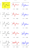
Fig 2. Example E2.

PCC and DTW_s versus the reference series r for the 15 time series $r_s^{\left[k\right]}\left(i\right)$ with s = 0, 5, 10, 20, 40 and k = 0, 1, 2. Each row corresponds to a different value of S, indicated by the figure in the top right corner of the plot in the first column. Each column corresponds to a different value of k: 0 on the left, with black curves, 1 in the centre, with blue curves and 2 on the right, with red curves. The plot in the top left panel with yellow background is the reference time series $r_0^{\left[0\right]}=r$. Under each panel, the corresponding values are reported for P(s, k) (italic) and D(s, k) (boldface).

Fig 3. Example E2.

PCC and DTW_s versus the reference series r for the $\left\{r_s^{\left[k\right]}\right\}$ with k = 0, 1, 2 and the time shift s ranging between 0 and 40. Squares correspond to P(s, k), while circles and solid lines indicate D(s, k); the different noise levels k = 0, 1, 2 are denoted by curves in black, blue and red respectively. The dashed lines in the bottom panel indicate the no-information value for DTW_s based on the null model described in Example ${\mathcal{E}}_2$.

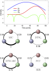
Fig 4. Example E3.

Plots (top) and PCC, MIC, DTW_s and DTW-MIC weighted coexpression networks (bottom) for the set $\mathcal{G}$ of the three time series G₁, G₂ and G₃ (in red, blue and green respectively). Arc width is proportional to edge weight.

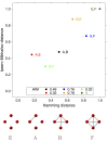
Fig 5. Example E4.

Mutual HIM distances in the H×IM space between 4 non-isospectral graphs A, B, E, F on 4 vertices, whose topology is shown below the plot. Distance values are listed in the plot legend.

Fig 6. GeneNetWeaver time series.

examples of 4 longitudinal expression level data generated by the GNW kinetic model for the synthetic subgraph of Yeast and E. coli regulatory networks. Time course data are defined on 41 time points 0, …, 1000 and they correspond to the genes YFR030W (black, from Yeast₂₀), YNL221C (green, from Yeast₂₀ with dual gene knockout), rhaS (from Ecoli₂₀) and putA (from Ecoli₅₀).

Fig 7. GeneNetWeaver data.

example of network reconstruction and comparison with the true network. In the top panels, the topology of the synthetic true network Yeast₂₀ (top left) is shown together with the Systematic Name of its 20 genes (top right). In the two bottom panels, the network Yeast₂₀ as inferred from the time course dataset d₁ by PCC (middle left), DTW-MIC (middle right), TimeDelay ARACNE (bottom left) and Transfer Entropy (bottom right). For the reconstructed networks, edge width is proportional to arc weight; edges with smaller weights (threshold is 0.001 for PCC, 0.135 for DTW-MIC and 0.005 for Transfer Entropy) are not drawn to avoid cluttering the image. Distance from the true network is 0.57 for the inference by PCC, 0.22 for the reconstruction by DTW-MIC, 0.28 for TimeDelay ARACNE and 0.57 for Transfer Entropy.

Fig 8. GeneNetWeaver data.

box and whisker plot of the HIM distance between the networks inferred from time series and the true graphs, listed in Table 1. For each true network Yeast₂₀, Ecoli₂₀ and Ecoli₅₀, 10 different graphs are reconstructed by PCC, DTW-MIC, TimeDelay ARACNE and Transfer Entropy similarity measures.

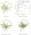
Fig 9. The T-cell example: True and DTW-MIC network.

The (true) network as reconstructed by Opgen-Rhein and Strimmer [128] (top left); the time course for three example genes EGR1 (blue), CD69 (red) and SCYA2 (orange), from replicate 1 of the tcell.34 (circles) and of the tcell.10 (squares) dataset. In the second row, the networks inferred by DTW-MIC from the tcell.10 (left) and from the tcell.34 (right) dataset; in these last two graphs, edges with weight smaller than 0.225 are not displayed.

Fig 10. The T-cell example: comparison networks.

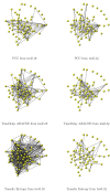
The Human t-cell network as reconstructed by PCC (top row), TimeDelay ARACNE (middle row) and Transfer Entropy (bottom row), from the tcell.10 (left column) and from the tcell.34 (right column) dataset. Edges with weights smaller than 0.1 for PCC and smaller than 0.0001 for Trasfer Entropy are not displayed.

Fig 11. Metric multidimensional scaling of HIM distances.

Planar projection conserving the mutual distances between the true Human t-cell network (TN) and the eight networks inferred from the two datasets tcell.34 (⋅₃₄) and tcell.10 (⋅₁₀) by the four reconstruction algorithms DTW-MIC (D), PCC (P), Transfer Entropy (T) and TimeDelay ARACNE (A).

References

1. De Smet R, Marchal K. Advantages and limitations of current network inference methods. Nat Rev Microbiol. 2010;8(10):717–729. - PubMed
1. Marbach D, Prill RJ, Schaffter T, Mattiussi C, Floreano D, Stolovitzky G. Revealing strengths and weaknesses of methods for gene network inference. Proc Natl Acad Sci USA. 2010;107(14):6286–6291. 10.1073/pnas.0913357107 - DOI - PMC - PubMed
1. Szederkenyi G, Banga J, Alonso A. Inference of complex biological networks: distinguishability issues and optimization-based solutions. BMC Syst Biol. 2011;5(1):177 10.1186/1752-0509-5-177 - DOI - PMC - PubMed
1. Allen JD, Xie Y, Chen M, Girard L, Xiao G. Comparing Statistical Methods for Constructing Large Scale Gene Networks. PLOS ONE. 2012;7(1):e29348 10.1371/journal.pone.0029348 - DOI - PMC - PubMed
1. López-Kleine L, Leal L, López C. Biostatistical approaches for the reconstruction of gene co-expression networks based on transcriptomic data. Brief Funct Genomics. 2013;12(5):457–467. 10.1093/bfgp/elt003 - DOI - PubMed
MeSH terms
LinkOut - more resources