Six Degrees of Auditory Spatial Separation

Abstract

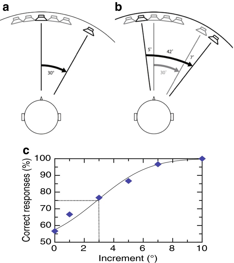
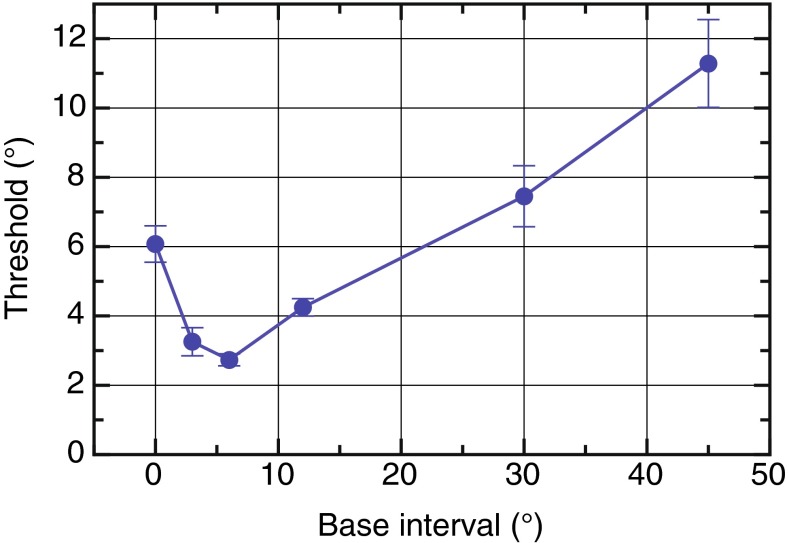
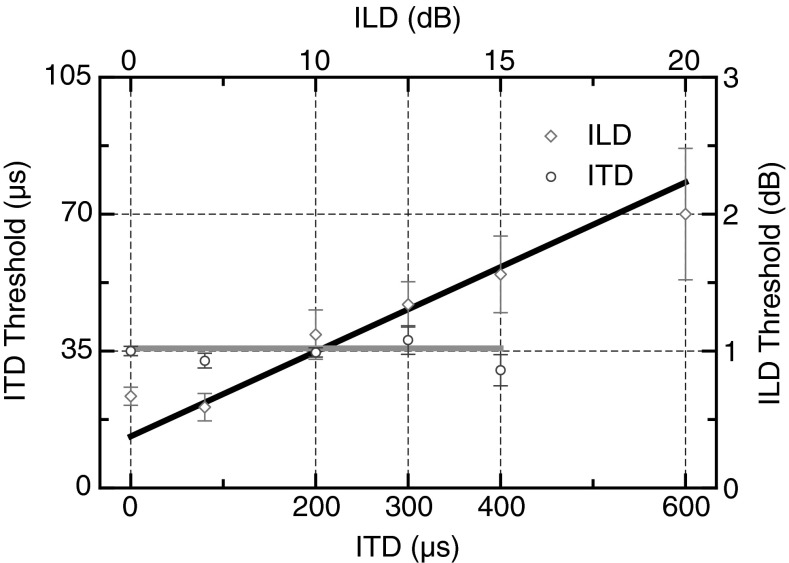
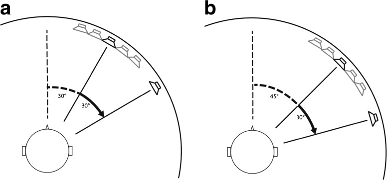
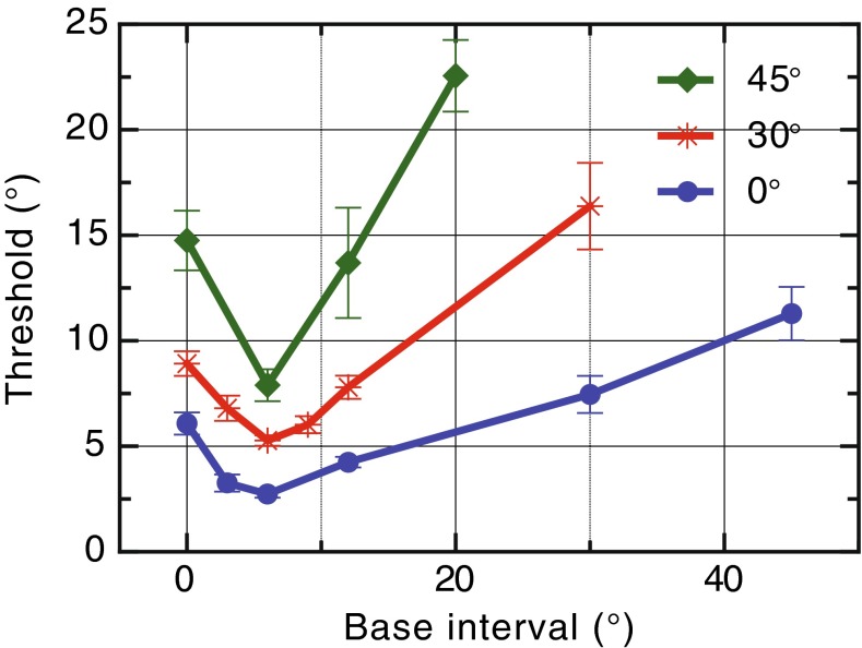
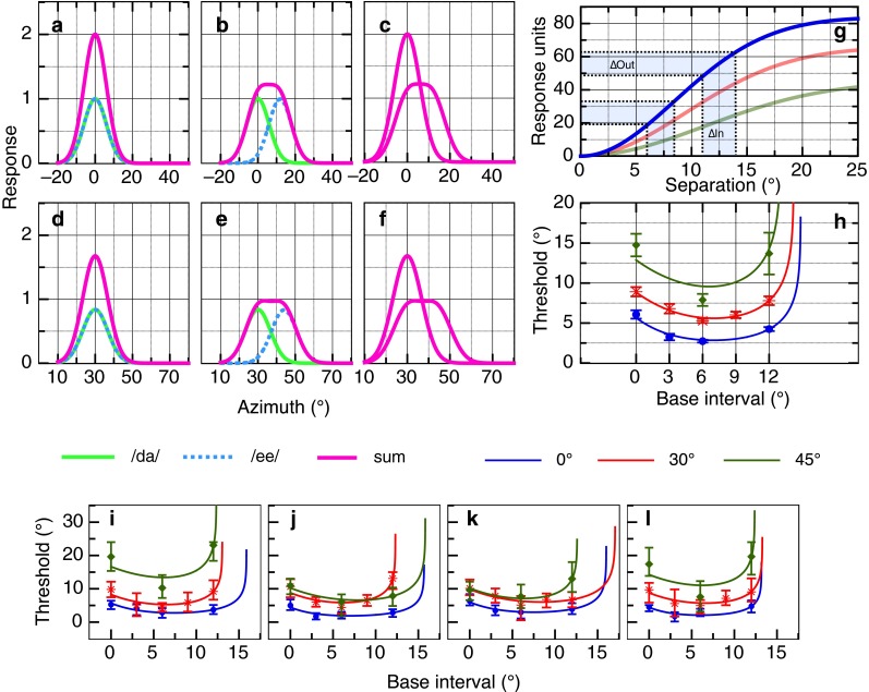
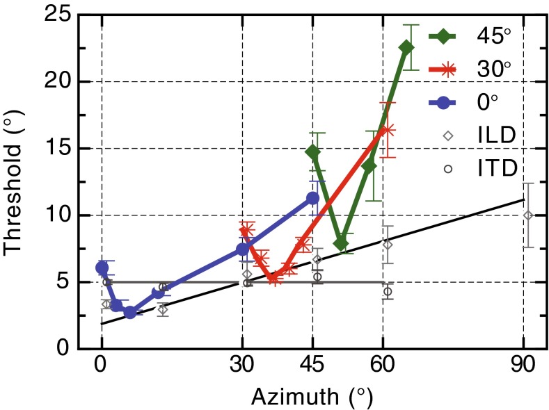
The location of a sound is derived computationally from acoustical cues rather than being inherent in the topography of the input signal, as in vision. Since Lord Rayleigh, the descriptions of that representation have swung between "labeled line" and "opponent process" models. Employing a simple variant of a two-point separation judgment using concurrent speech sounds, we found that spatial discrimination thresholds changed nonmonotonically as a function of the overall separation. Rather than increasing with separation, spatial discrimination thresholds first declined as two-point separation increased before reaching a turning point and increasing thereafter with further separation. This "dipper" function, with a minimum at 6 ° of separation, was seen for regions around the midline as well as for more lateral regions (30 and 45 °). The discrimination thresholds for the binaural localization cues were linear over the same range, so these cannot explain the shape of these functions. These data and a simple computational model indicate that the perception of auditory space involves a local code or multichannel mapping emerging subsequent to the binaural cue coding.

Keywords: auditory localization; auditory spatial perception; sensory channel processing.

FIG. 1

A, B Schematic of the experimental setup for the anterior field, as viewed from directly above the listener. A fixed array of five speakers, each separated by 5 °, and a single speaker attached to a movable robotic arm (black outer circle) are located in front of the participant. In each interval, participants are concurrently presented two spatially separated sounds. Participants reported the interval that contained the wider spatial separation. A An example standard interval: /da/ is presented at 0 ° using the middle speaker in the array and /ee/ 30 ° to the right of the midline using the speaker on the movable arm. This produces a spatial separation of 30 °, the base separation in this trial. Active speakers and their sound direction lines are in black and inactive speakers are in gray. B An example test interval: /da/ is presented 5 ° to the left of the midline using a fixed speaker and /ee/ is presented 37 ° to the right of the midline using the speaker on the movable arm. This results in a spatial separation of 42 °, which corresponds to an increment of 12 ° on the base separation of 30 °. The gray lines show the spatial separation in the previous interval. The left and right endpoints were varied across trials and neither was ever in the same location, preventing participants reporting a change in the location of one of the tokens. C Data from a representative subject for a single base separation in the free-field task. The percentage of correct responses is plotted as a function of the increment presented, with each point representing the average of 18 trials. The line shows the best-fitting cumulative Gaussian function from which thresholds are calculated. The dotted lines show the increment corresponding to 75 % correct performance.

FIG. 2

Overall mean increment discrimination thresholds in the free-field task as a function of the base interval.

FIG. 3

Overall mean increment discrimination thresholds for the single-source ITD and ILD tasks as a function of the baseline ITD or ILD offset. All error bars are ±1 SEM.

FIG. 4

A, B Schematic of the experimental setup for eccentric regions of space. A The fixed array is located 30 ° to the right of the midline. B The fixed array is located 45 ° to the right of the midline.

FIG. 5

Overall mean increment thresholds as a function of the base separation for each of the eccentric conditions.

FIG. 6

Proposed model for free-field spatial separation discrimination. A Two collocated responses (blue and green) located at lateral offset of 0 ° each of magnitude 1, the sum forms a single peak of amplitude 2.0 (magenta line). B Two spatially separated responses (blue and green); the summed response forms a flattened peak (magenta line). C The summed Gaussian responses taken from A and B. D Two collocated responses located at a lateral offset of 30 ° as in A but each with a magnitude of 0.8. E Two spatially separated responses as in B. F The summed Gaussians taken from D and E. The effect of the gain (attenuation) factor for more eccentric location can be seen by the reduction in amplitude of the responses D–F, with the summed response reaching a maximum of 1.6. G The summed Gaussian responses (magenta lines) in C are subtracted from each other, and the sum of the square of this difference is taken across all azimuth values. This produces a sigmoidal pattern of accelerating nonlinearity followed by compressive nonlinearity (blue curve). The red curve shows this computation for F and the green curve for an eccentricity of 45 ° (summed Gaussians not illustrated). H Measured thresholds and predictions from the model. Thresholds were simulated by assuming correct discrimination requires a constant change in response output from the functions shown in (G—e.g., blue shading). I–L Predicted and measured thresholds for four participants who completed all three lateral offset conditions. All error bars are 95 % confidence intervals. See text for further details.

FIG. 7

Overall mean increment thresholds for the free-field and binaural cue tasks as a function of eccentricity in degrees azimuth from the midline. The increment thresholds for the binaural cues have been converted to an equivalent threshold in degrees. All error bars are ±1 SEM.

References

1. Ahveninen J, Kopco N, Jaaskelainen IP. Psychophysics and neuronal bases of sound localization in humans. Hear Res. 2014;307:86–97. doi: 10.1016/j.heares.2013.07.008. - DOI - PMC - PubMed
1. Ashida G, Carr CE. Sound localization: Jeffress and beyond. Curr Opin Neurobiol. 2011;21:745–751. doi: 10.1016/j.conb.2011.05.008. - DOI - PMC - PubMed
1. Best V, Schaik A, Carlile S. Separation of concurrent broadband sound sources by human listeners. J Acoust Soc Am. 2004;115:324–336. doi: 10.1121/1.1632484. - DOI - PubMed
1. Best V, Ozmeral E, Gallun FJ, Sen K, Shinn-Cunningham BG. Spatial unmasking of birdsong in human listeners: energetic and informational factors. J Acoust Soc Am. 2005;118:3766–3773. doi: 10.1121/1.2130949. - DOI - PubMed
1. Bizley JK, Cohen YE. The what, where and how of auditory-object perception. Nat Rev Neurosci. 2013;14:693–707. doi: 10.1038/nrn3565. - DOI - PMC - PubMed
LinkOut - more resources