Functional network inference of the suprachiasmatic nucleus

Abstract

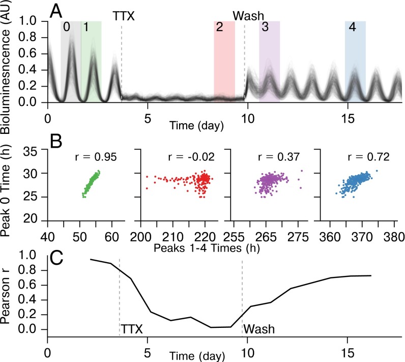
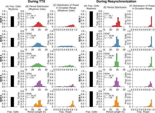
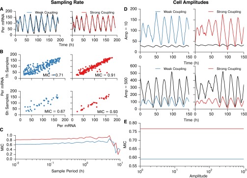
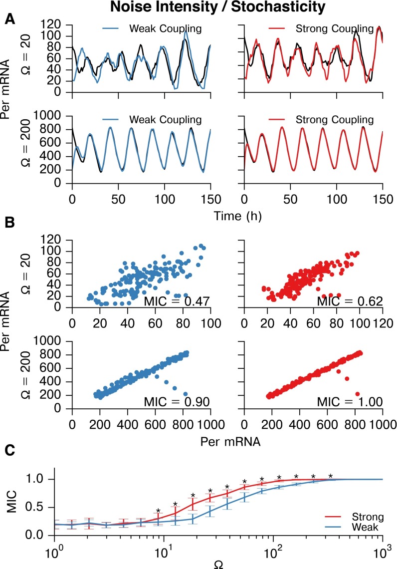
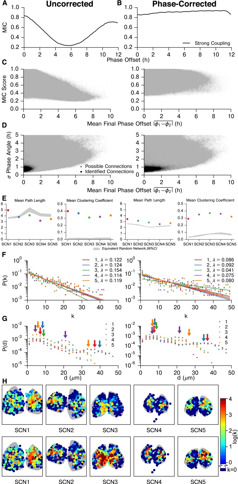
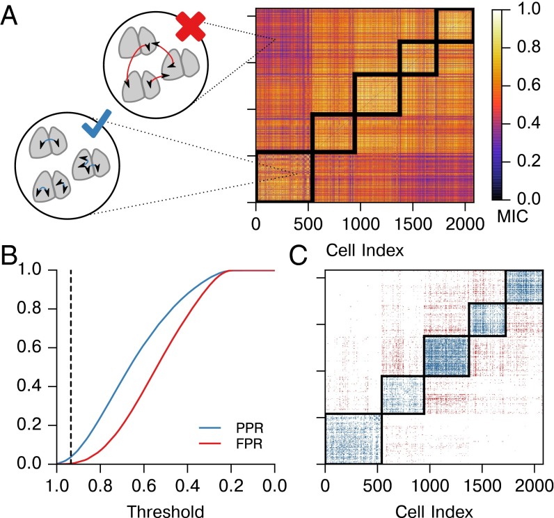
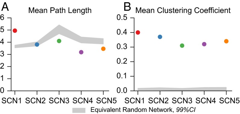
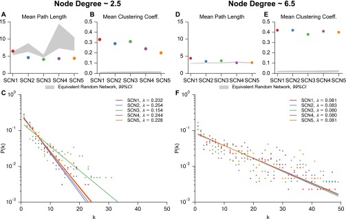
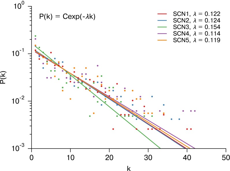
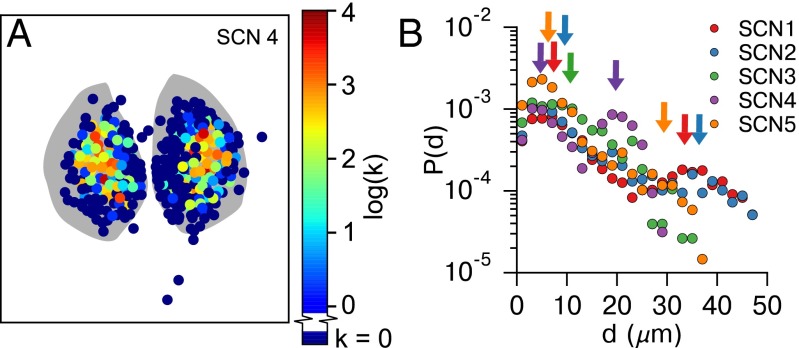
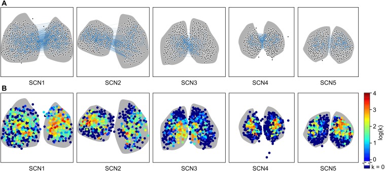
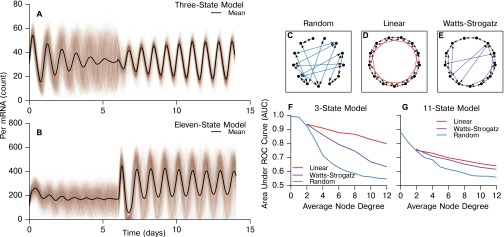
In the mammalian suprachiasmatic nucleus (SCN), noisy cellular oscillators communicate within a neuronal network to generate precise system-wide circadian rhythms. Although the intracellular genetic oscillator and intercellular biochemical coupling mechanisms have been examined previously, the network topology driving synchronization of the SCN has not been elucidated. This network has been particularly challenging to probe, due to its oscillatory components and slow coupling timescale. In this work, we investigated the SCN network at a single-cell resolution through a chemically induced desynchronization. We then inferred functional connections in the SCN by applying the maximal information coefficient statistic to bioluminescence reporter data from individual neurons while they resynchronized their circadian cycling. Our results demonstrate that the functional network of circadian cells associated with resynchronization has small-world characteristics, with a node degree distribution that is exponential. We show that hubs of this small-world network are preferentially located in the central SCN, with sparsely connected shells surrounding these cores. Finally, we used two computational models of circadian neurons to validate our predictions of network structure.

Keywords: biological clock; circadian oscillator; mathematical model; synchronization; systems biology.

Fig. 1.

Experimental protocol demonstrating TTX-mediated resynchronization for SCN1. (A) Bioluminescence traces from individual cells within SCN1, showing pre-TTX, during-TTX, and post-TTX single-cell oscillations. (B) In the functioning SCN, peak times are highly correlated from cycle to cycle. We compare relative peak times 1 (pre-TTX), 2 (during-TTX), and 3–4 (post-TTX), to the first peak (0) to show that a resynchronization is indeed taking place and that the SCN network structure reverts to pre-TTX structure slowly after TTX wash. (C) Plot of Pearson r for correlating each peak to peak 0, showing the resynchronization. Pearson r does not completely return to pre-TTX levels due to inability to track cells accurately across TTX conditions.

Fig. S1.

Summary statistics for SCN slices during TTX application and during resynchronization. (A and D) Fraction of cells which displayed rhythmic circadian oscillation (A) during TTX or (D) during resynchronization. Not all cells observed during resynchronization could be tracked during TTX due to very low luminescence (as in ref. 36); cells that could not be tracked were classified as arrhythmic. We found that chemically uncoupled cells are nondeterministic, weak oscillators, in accordance with ref. . When recoupled after TTX washout, nearly all cells observed became rhythmic. A cell was determined to be rhythmic if it exhibited a Lomb–Scargle periodogram peak between the 18- and 32-h period at $P<0.05$ significance. Data were baseline detrended via discrete wavelet transform. (B and E) Period length histograms (B) during TTX application and (E) during resynchronization. As period varies cycle-to-cycle for decoupled oscillators and during resynchronization, we report each peak to peak period of oscillation for each cell, rather than finding the mean period of a cell through fitting a sinusoid. Peak times were identified by a discrete wavelet transform filtering for peaks with period between 16 and 32 h. (C and F) Histograms of the fraction of oscillatory power in the circadian frequency range (16–32 h) (C) during TTX or (F) during resynchronization, calculated via fast Fourier transform. Data were baseline detrended before FFT. We note that not all cells are observable during TTX due to low bioluminescence, and thus column C includes only rhythmic, observable cells. For all SCNs, the period distribution tightened and more oscillatory power was in the circadian range during resynchronization. As these effects and distributions are consistent across SCNs during resynchronization, a cross-comparison may be used to control FPR.

Fig. S2.

MIC score for identification of network connections is largely invariant with respect to sampling rate and amplitude. (A–C) Testing the effect of sampling rate on the ability to distinguish between strongly and weakly coupled simulated cells. We use strongly and weakly coupled cells rather than coupled and uncoupled cells because the entire SCN is indirectly coupled, and therefore we are only interested in the strongest connections. (D and E) MIC binning procedure effectively normalizes amplitude, and therefore raw amplitude has no effect on MIC score. (A) Per mRNA traces for two weakly coupled cells (Left; coupling strength parameter = 0.0033) and two strongly coupled cells (Right; coupling strength parameter = 0.010). For both simulations in A–C, the discrete stochastic three-state model (34) was used, with volume parameter $\text{Ω}$ = 40, and the simulation sampling rate was set to 100 samples/h. (B) Scatter plots and MIC values of Per mRNA for the cell pairs, downsampled to 1- or 6-h intervals. (C) Effect of sample interval on MIC score. For sampling intervals shorter than ∼2 h, only marginal changes in MIC are seen, indicating that the MIC score is largely consistent with increased sampling rate. For sampling intervals longer than 2 h (<10 samples/cycle), the MIC score becomes less accurate, and the ability to distinguish between connections of varying strength is reduced. (D) To demonstrate the effective normalization of cellular trajectories through MIC binning, we compared MIC values for strongly and weakly coupled cells while scaling the peak-to-trough amplitude. For both simulations in D and E, the sampling rate was set to 1 sample/h. Peak to trough amplitude of one of the resulting trajectories was scaled to $Amp=10$ (Upper) or $Amp=500$ (Lower) for visualization. (E) MIC score is completely invariant with respect to changes in amplitude of a simulated trajectory, as the gridding algorithm in MIC is effectively a normalization.

Fig. S3.

MIC is able to distinguish between strongly and weakly connected cells for a wide range of stochasticity. Stochastic noise in the three-state model (34) was tuned by changing the volume parameter $\mathrm{\Omega }$. Stochastic noise causes cells to drift in phase, and thus is essential for this inference. (A) Representative Per mRNA traces of weakly coupled (Left; coupling strength = 0.0033) and strongly coupled (Right; coupling strength = 0.010) cells resynchronizing for $\mathrm{\Omega }=20$ (Upper) and $\mathrm{\Omega }=200$ (Lower). For all simulations here, sampling intervals were 1 h, as in the experiment. (B) Scatter plots and MIC values of Per mRNA for these representative cell pairs at $\mathrm{\Omega }=20$ and $\mathrm{\Omega }=200$. (C) Plot of mean $\pm$ SD. MIC values for strongly and weakly coupled cell pairs vs. $\mathrm{\Omega }$ (n = 33 cell pairs at each $\mathrm{\Omega }$). A broad range of stochasticity allows differentiation between strong and weak coupling (^⋆P $<0.05$, Wilcoxon sign rank test with Bonferroni correction). At very low $\mathrm{\Omega }$ values, oscillation does not occur, and at very high $\mathrm{\Omega }$ values, the MIC scores for both pairs approach 1.0. The experimentall -determined $\mathrm{\Omega }=40$ is well within the range for which MIC can distinguish between connections.

Fig. S4.

Effect of phase offset on MIC network inference. MIC is not phase-agnostic, and so the question arises of whether the inferred functional networks are driven by phase distributions in each SCN, similar to the phase clusters identified in (19). First, we show how phase offset affects MIC score for pairs of synchronized oscillators. Next, we show that realigning out of phase trajectories and taking the maximum MIC reduces much of this bias. Finally, we examine how this affects the connections we identify in the five SCN tissues, and show that our results are consistent after applying this phase offset correction. (A) The MIC score varies with phase offset between two phase-locked oscillators. Each point on this plot was generated by simulating 50 pairs of strongly coupled cells, as in S2. Connected cells in this model synchronize to a phase offset of 0 h because they are parameterized identically. One trajectory from each pair was phase-shifted in 0.1-h increments up to 12 h, to generate a range of phase offsets between the trajectories. The mean MIC score (y axis) of the 50 pairs was then computed for each artificially created phase offset (x axis). As the phase offset between coupled cells is increased, the MIC score is reduced from its maximum at a 0-h angle. This is considered the uncorrected case, where MIC is computed with no regard for the phase offset between trajectories. (B) Next, we took the phase-shifted trajectories from A and performed a correction to renormalize MIC, so that MIC score is not affected by the phase offset between cells that we originally added. The correction was performed by again shifting the trajectories 12 h in either direction, this time in intervals of 1.0 h to reflect experimental sampling rate, and calculating MIC scores at each of these shifts. We then selected the largest of the resulting values as the MIC score for the cell pair, as this maximum MIC corresponds to when phases are realigned. In comparison with the uncorrected method, the maximum MIC correction results in reduced sensitivity to the phase offset between cells, as the corrected MIC score (y axis) is nearly flat with respect to the phase offset of the pair (x axis). This method reduces power, however, as some of the initial resynchronization period must be truncated to realign phases, resulting in a slight bias toward larger phase offsets. Thus, the uncorrected method (biased toward small phase offset) and corrected maximum MIC method (slightly biased toward large phase offset) form bounds on connectivity. (C) Scatter plot of MIC score vs. mean phase offset for all possible connections within each SCN. There is a clear bias against absolute phase offsets greater than $\sim 2$ h (Left), in a similar form as A. This bias is rectified by performing the maximum MIC correction (Right). Phase offset (used only for plotting purposes) was calculated by a Hilbert transform after removing the trend via discrete wavelet baseline detrending. As the phase offset was unstable early during resynchronization, it was calculated after it had stabilized, during days 6–7. (D) Plot of SD of phase offset vs. mean phase offset for possible and identified connections within all five SCNs. SD of phase offset was calculated throughout the resynchronization period, and can be thought of as a measure of phase offset instability between two cells. As expected, MIC detects connections between cells with a low SD in phase offset for both cases, with a wider range of mean phase offsets. Thresholds were raised for each of the five SCNs (to 0.980, 0.970, 0.999, 0.985, and 0.985, respectively) after phase correction, as all MIC scores are increased by this method. Generally, cell pairs with a larger phase offset also had a less stable phase offset, such that even after phase offset correction most connections were between cells with a difference in phase of less than 2 h. (E) Phase-corrected SCN networks maintained small-world characteristics, with a comparable mean path length and larger clustering coefficient than corresponding random networks. (F) Node degree distributions for each SCN remain exponential (P < 0.0001 for each SCN, likelihood-ratio test comparison with power law fits), although λ changes corresponding to the increased average node degree for SCNs in which phases were aligned. SCN 3 deviates slightly from the others here, due to the high number of connections which yield saturated (1.0) MIC scores after realignment. (G) Connection length distributions for unaligned and phase-aligned networks. Despite the higher average node degree for aligned networks, these distributions continued to display two peaks: one for local connections within a core, and a second corresponding to core-core connections. (H) Similarly, core-shell hierarchy was maintained after phase-alignment. Additionally, many shell neurons remain functionally unconnected, indicating a much slower resynchronization than neurons in SCN core regions. These neurons do synchronize; however, they are less tightly synchronized than cells which have identifiable connections.

Fig. 2.

MIC identifies the strongest connections within a whole SCN sample. (A) Here, we calculate and plot pairwise MIC between neurons from all SCNs. We consider connections within the same SCN to be valid, whether between halves or within a single half. Connections between physiologically distinct SCNs are invalid, as they are biologically infeasible. The block-diagonal regions outlined in black contain valid connections, and connections outside of this region are invalid. (B) False-positive rate (FPR, red, inter-SCN connections) and possible positive rate (PPR, blue, same-SCN connections) are plotted for varying MIC threshold values. We choose an initial threshold of 0.935, for which FPR = 0.0032. (C) The connections identified by applying the threshold from B are shown to occur primarily in biologically valid areas (blue), with few invalid connections found (red). Thus, the strongest functional connections within each SCN are identified.

Fig. 3.

SCN functional networks display small-world structure. (A) Average path length is on the same order of magnitude of an equivalent random (Erdos-Renyi) network. (B) Clustering coefficient is a magnitude greater than that of equivalent randomly generated networks. CIs are determined by generation of 10,000 equivalent Erdos-Renyi networks for each SCN.

Fig. S5.

Small-world network characteristics and discrete exponential distribution of node degree is insensitive to selected MIC threshold. Threshold was altered for each SCN to yield an average node degree of ∼2.5 (A–C) and 6.5 (D–F). (A and D) Average path length remains on the same order of magnitude as that of an equivalent random network (99% CI taken from 10,000 randomly generated networks). (B and E) Average clustering coefficient remains an order of magnitude higher than that of an equivalent randomly generated network, confirming small-worldness. (D and F) Node degree distribution remains exponential for average node degrees of 2.5 and 6.5. As in Fig. 4, the resulting discrete exponential distributions $P\left(k\right)=C\exp \left(-\text{λ}k\right)$ were fit via numerical optimization of the maximum likelihood, resulting in distribution parameters λ for each network. Each SCN is better fit by a discrete exponential distribution than a discrete power law distribution (likelihood-ratio test, $P<0.0005$ for each SCN). SCN3 lacks sufficient resolution to lower node degree below $\sim$ 4.0, and therefore shows slight deviation in λ for low average node degree.

Fig. 4.

Node degree (k) distributions for SCNs 1–5 plotted on a semilog scale. The resulting discrete exponential distributions $P\left(k\right)=C\exp \left(-\text{λ}k\right)$ were fit via numerical optimization of the maximum likelihood, resulting in distribution parameters λ for each network. Each SCN is better fit by a discrete exponential distribution than a discrete power law distribution (likelihood-ratio test, $P<0.0005$ for each SCN). The strong agreement between λ shows a consistent network structure across SCNs. This agreement exists for a range of node degrees (Fig. S5).

Fig. 5.

Hubs of the small-world network are located in the central SCN. (A) Heatmap of node degree [color $\propto \text{log}\left(k\right)$] distribution for a representative SCN shows that hubs of the small-world network are preferentially located in SCN core regions. All SCNs are shown in Fig. S6. (B) Connection length (d μm) distributions for SCNs 1–5 plotted on a semilog scale. Two peaks (arrows) are identifiable for SCNs 1, 2, 4, and 5: a local peak corresponding to connections between physically nearby neurons, and a second peak corresponding to the distance for functional connections between central SCN regions. For SCN3, these peaks are indistinguishable due to lack of spatial separation between cores.

Fig. S6.

Hubs of the small-world network are located in the central SCN. (A) Inferred networks are shown overlaid on SCN tissue shape (gray). Connections between nodes are particularly dense in core regions and individual connections are difficult to distinguish. The third ventricle is oriented at the top of each network. Strong functional connections between halves indicate that the core regions communicate to establish consistent phase to entrain the shell. Cells which have no or few functional connections are preferentially located in the outer SCN shell regions. (B) Heatmaps of node degree [color $\propto \text{log}\left(k\right)$] distribution show that hubs of the small-world network are preferentially located in SCN core regions.

Fig. S7.

Accuracy of the MIC inference method depends on both network topology and average node degree. (A and B) Representative simulations capturing the TTX-mediated resynchronization for the 3-state and 11-state models, respectively. Next, MIC network inference was performed for simulated networks of three topologies: (C) random, (D), linear nearest neighbor, and (E) Watts–Strogatz small world ($\text{β}=0.05$). These networks are only shown for visualization of network structure. Simulated networks each contained 400 cells to match SCN recordings, and the average AUC was calculated for five dynamically generated networks of each node degree. The area under the ROC curve is plotted as a function of average node degree for the 3-state circadian model (33, 34) (F) and the 11-state circadian model (35) (G) for these network structures. We show that both node degree and network structure affect the accuracy of this method. In general, networks that have a shorter average path length and higher average node degree are more difficult to accurately infer, as it becomes increasingly difficult to differentiate between direct and indirect physical connections.

Fig. S8.

ROC curve ranges and mean AUC values for simulation and inference of the SCN networks with physical connections dictated by the functional network, using (A) the 3-state (33, 34) and (B) the 11-state (35) models. Shaded ranges were calculated from seven simulations using unique random seeds. We note that all neurons are simulated, including those which are unconnected. Unconnected neurons do synchronize experimentally, although at a slower rate. To reflect this, unconnected cells in simulation were connected to the mean field, but at a reduced coupling strength. Errors in this method are largely incurred by secondary connections within tightly coupled regions (i.e., physical connections of cell 1$\to$ cell 2$\to$cell 3 often show the additional cell 1$\to$cell 3 functional connection).

References

1. Refinetti R, Menaker M. The circadian rhythm of body temperature. Physiol Behav. 1992;51(3):613–637. - PubMed
1. Nagoshi E, et al. Circadian gene expression in individual fibroblasts: Cell-autonomous and self-sustained oscillators pass time to daughter cells. Cell. 2004;119(5):693–705. - PubMed
1. Bieler J, et al. Robust synchronization of coupled circadian and cell cycle oscillators in single mammalian cells. Mol Syst Biol. 2014;10:739. - PMC - PubMed
1. Sassone-Corsi P. Molecular clocks: Mastering time by gene regulation. Nature. 1998;392(6679):871–874. - PubMed
1. Bass J, Takahashi JS. Circadian integration of metabolism and energetics. Science. 2010;330(6009):1349–1354. - PMC - PubMed
Publication types