Importance of ocean salinity for climate and habitability

Abstract

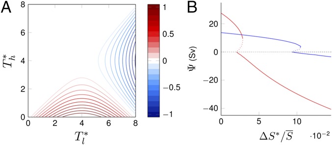
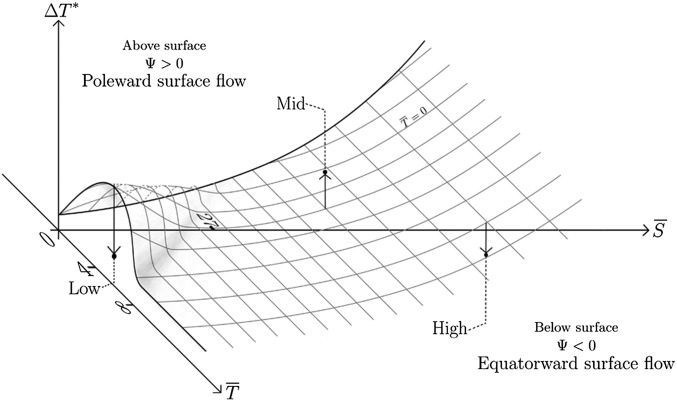
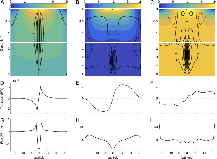
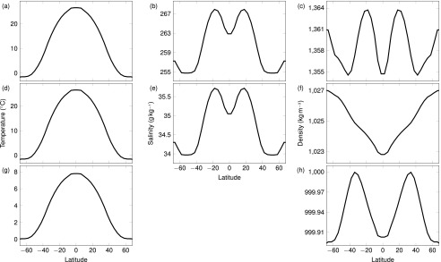
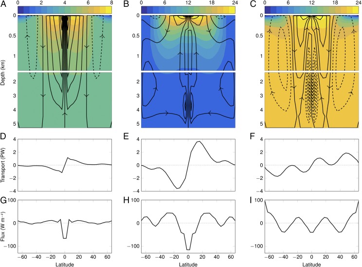
Modeling studies of terrestrial extrasolar planetary climates are now including the effects of ocean circulation due to a recognition of the importance of oceans for climate; indeed, the peak equator-pole ocean heat transport on Earth peaks at almost half that of the atmosphere. However, such studies have made the assumption that fundamental oceanic properties, such as salinity, temperature, and depth, are similar to Earth. This assumption results in Earth-like circulations: a meridional overturning with warm water moving poleward at the surface, being cooled, sinking at high latitudes, and traveling equatorward at depth. Here it is shown that an exoplanetary ocean with a different salinity can circulate in the opposite direction: an equatorward flow of polar water at the surface, sinking in the tropics, and filling the deep ocean with warm water. This alternative flow regime results in a dramatic warming in the polar regions, demonstrated here using both a conceptual model and an ocean general circulation model. These results highlight the importance of ocean salinity for exoplanetary climate and consequent habitability and the need for its consideration in future studies.

Keywords: exoplanet; habitability; ocean circulation; planetary climate.

Fig. 1.

Box model solutions for the magnitude of the overturning circulation $\mathrm{\Psi }$ (Sv = 10⁶ m³⋅s⁻¹) for the three salinity scenarios. (A) Freshwater case with surface temperature forcing $T_h^{\text{∗}}$ and $T_l^{\text{∗}}$ (°C), of the high and low latitude box, respectively, in the range 0–8 °C, contour interval 0.1 Sv. Positive circulation occurs when $T_h^{\text{∗}}<T_l^{\text{∗}}<8-T_h^{\text{∗}}$ (assuming $T_h^{\text{∗}}<T_l^{\text{∗}}$). (B) Mid- (blue) and high (red) range salinity scenarios, dotted lines indicate unstable solutions, $\mathrm{\Delta }{S}^{\text{*}}$ is the gradient in salinity forcing, and $\overline{S}$ is the mean salinity. The scaling $\mathrm{\Delta }{S}^{\text{*}}\propto \overline{S}$ means direct comparison is possible when $\mathrm{\Delta }{S}^{\text{*}}/\overline{S}$ is varied. The range presented is equivalent to 0–5 and 0–38 g⋅kg⁻¹ for $\mathrm{\Delta }{S}^{\text{*}}$ in the midrange and high range salinity cases, respectively. A salinity-driven circulation occurs when $\mathrm{\Delta }{S}^{\text{*}}/\overline{S}>$ 0.105 and 0.03, respectively.

Fig. 2.

A schematic illustrating the direction and magnitude of the overturning circulation, $\mathrm{\Psi }$, from the box model solutions. The behavior depends on the values of temperature gradient forcing $\mathrm{\Delta }{T}^{\text{*}}$, the mean temperature $\overline{T}$, and mean salinity $\overline{S}$. The proportionality between the salinity gradient forcing $\mathrm{\Delta }{S}^{\text{*}}$ and $\overline{S}$ means the two values do not need separate consideration, whereas $\mathrm{\Delta }{T}^{\text{*}}$ and $\overline{T}$ can be varied independently. Note the lower limit of $\overline{T}$ decreases as $\overline{S}$ increases and lowers the freezing point. Values lying on the surface have zero circulation $\mathrm{\Psi }=0$; those above and below have positive and negative circulation, respectively, with increasing magnitude with increasing distance from the surface. The values defining the low-salinity, low-temperature range are indicated; 0–8 °C and 0–27 g⋅kg⁻¹, with the local maximum at $\overline{T}=$ 4 °C, $\overline{S}=$ 0 g⋅kg⁻¹. The locations of the low, mid-, and high salinity ranges considered in this study are indicated in reference to the surface. The curvature of the surface results from the nonlinear dependence of density on temperature and salinity.

Fig. 3.

Plots showing the results from the OGCM for the freshwater (A, D, and G), mid- (B, E, and H), and high (C, F, and I) range salinity scenarios; note the different scales in A, D, and G. (A–C) Black contours of the overturning streamfunction $\mathrm{\Psi }$ show the structure of the meridional overturning circulation through the depth of the ocean. The contour intervals are (A) 1 Sv (=10⁶ m³⋅s⁻¹) and (B and C) 20 Sv. Solid and dashed contours indicate positive (poleward surface flow) and negative (equatorward surface flow) circulation, respectively, as indicated by the arrows. Note the different depth scales; the surface layer is extended to show this region of finer detail; the color shading in A–C shows the zonally averaged temperature (°C). (D–F) Northward ocean heat transport (PW = 10¹⁵ W). (G–I) Surface heat flux (W⋅m⁻²); positive values are from ocean to atmosphere.

Fig. S1.

Plots showing the zonally averaged profiles of atmospheric temperature (A, D, and G) and salinity (B and E) forcing on the surface of the ocean in the OGCM, for the high (A–C) and mid- (D–F) range salinity scenarios, and the freshwater case (G and H). Note there is no salinity forcing in the freshwater case. The density forcing (C, F, and H) is calculated from the temperature and salinity values shown using the relevant equation of state.

Fig. 4.

Plots showing the results from the OGCM for the freshwater (A, D, and G), mid- (B, E, and H), and high (C, F, and I) range salinity scenarios with the inclusion of wind forcing. (A–C) Black contours of the overturning streamfunction $\mathrm{\Psi }$ show the structure of the meridional overturning circulation through the depth of the ocean; the contour interval is 20 Sv (=10⁶ m³⋅s⁻¹). Solid and dashed contours indicate positive (poleward surface flow) and negative (equatorward surface flow) circulation, respectively, as indicated by the arrows. Note the different depth scales; the surface layer is extended to show this region of finer detail. The color shading in A–C shows the zonally averaged temperature (°C); note the different scale in A. (D–F) Northward ocean heat transport (PW = 10¹⁵ W). (G–I) Surface heat flux (W⋅m⁻²); positive values are from ocean to atmosphere.

References

1. Dole SH. Habitable Planets for Man. Blaisdell; New York: 1964.
1. Kasting JF, Whitmire DP, Reynolds RT. Habitable zones around main sequence stars. Icarus. 1993;101(1):108–128. - PubMed
1. Heller R, Armstrong J. Superhabitable worlds. Astrobiology. 2014;14(1):50–66. - PubMed
1. Showman AP, Wordsworth RD, Merlis TM, Kaspi Y. Atmospheric circulation of terrestrial exoplanets. In: Mackwell SJ, et al., editors. Comparitive Climatology of Terrestrial Exoplanets. Univ. of Arizona; Tucson: 2013. pp. 277–326.
1. Williams GP. The dynamical range of global circulations–I. Clim Dyn. 1988;2(4):205–260.
Publication types
LinkOut - more resources