Robust neuronal dynamics in premotor cortex during motor planning

Abstract

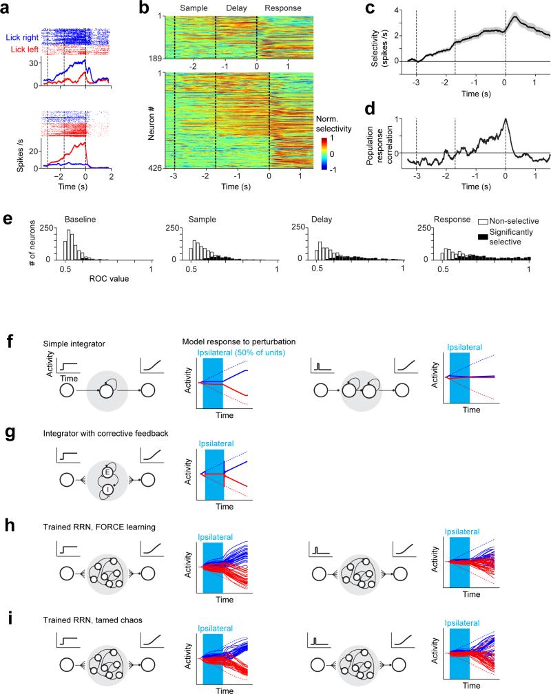
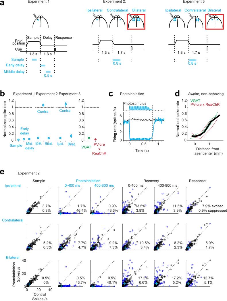
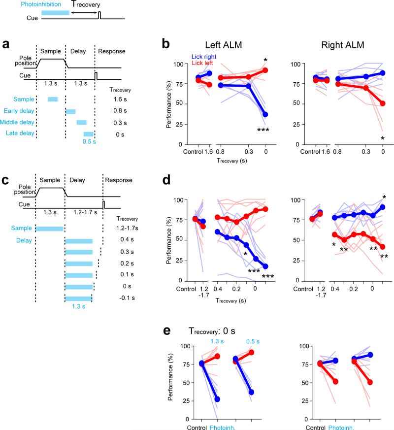
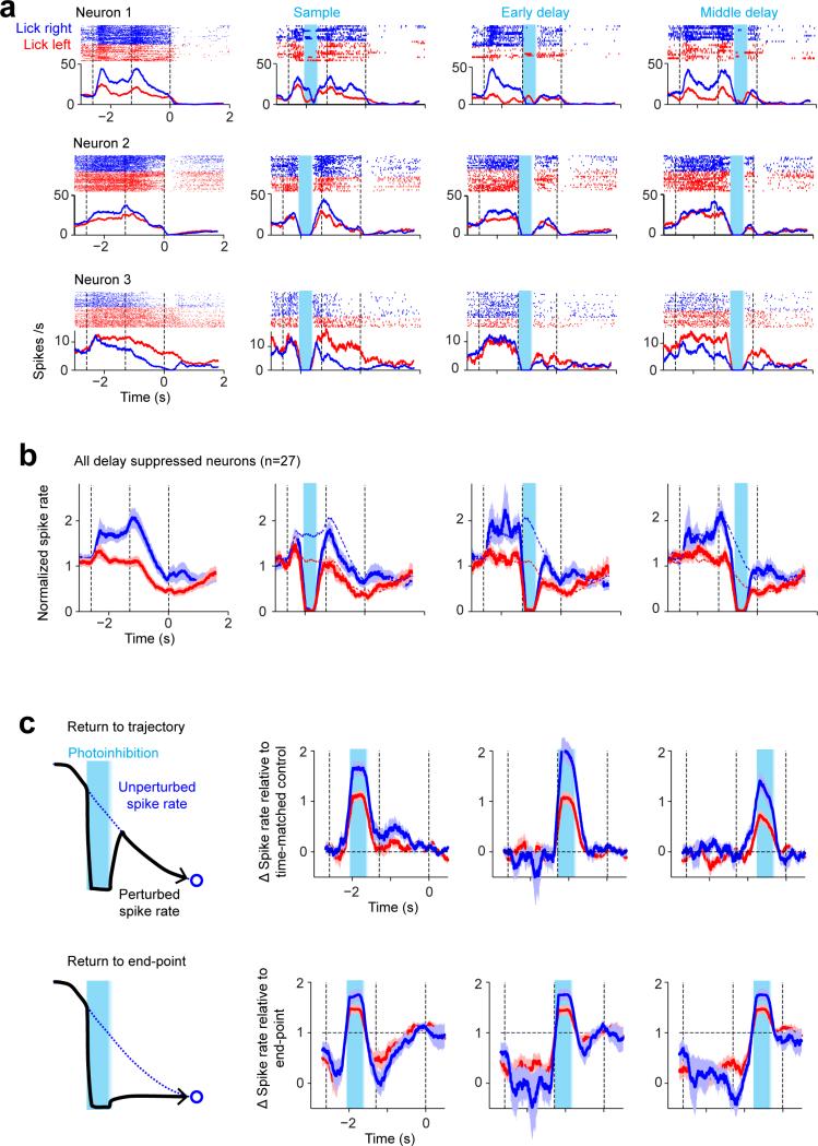
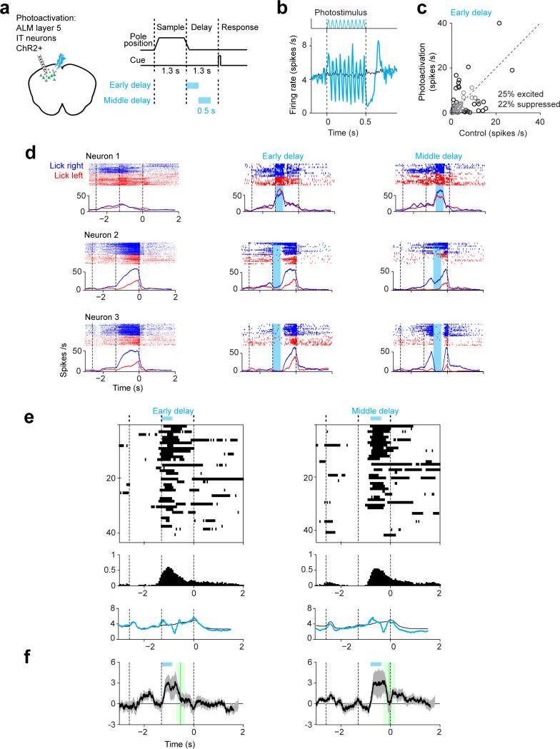
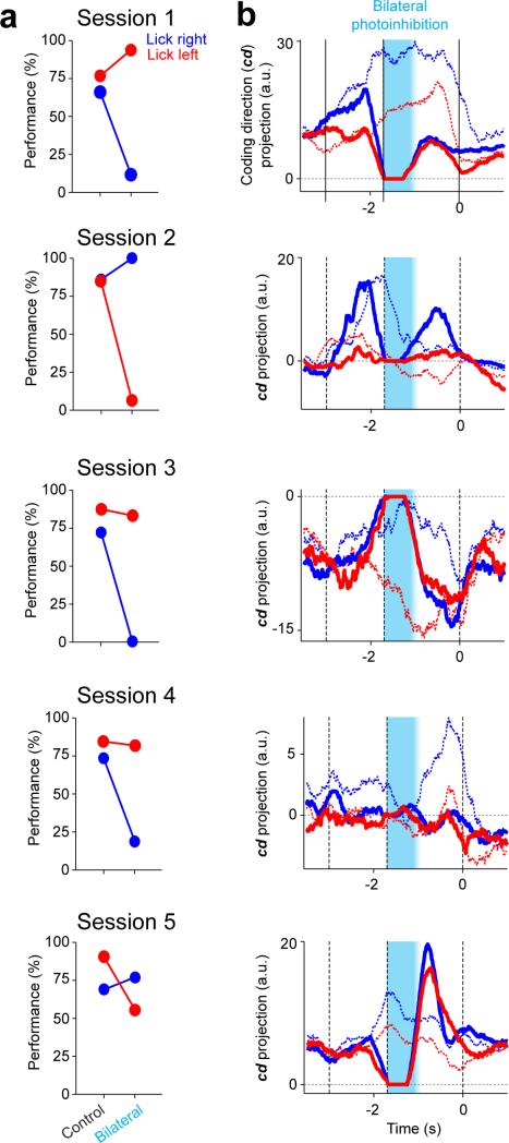
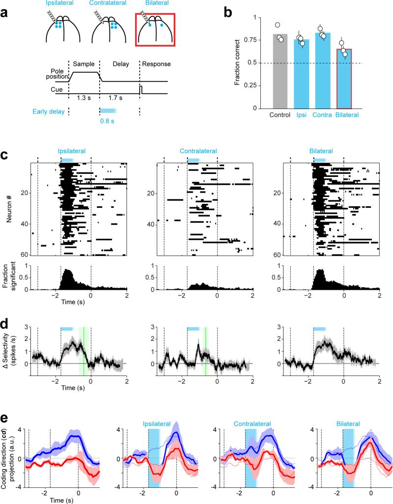
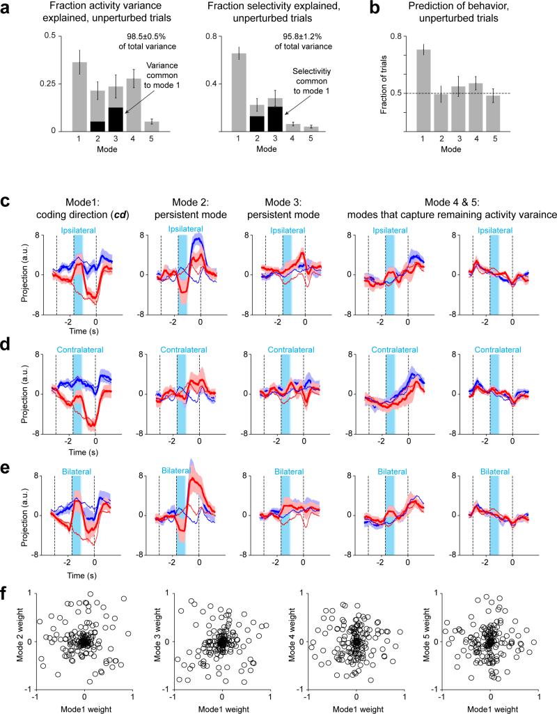
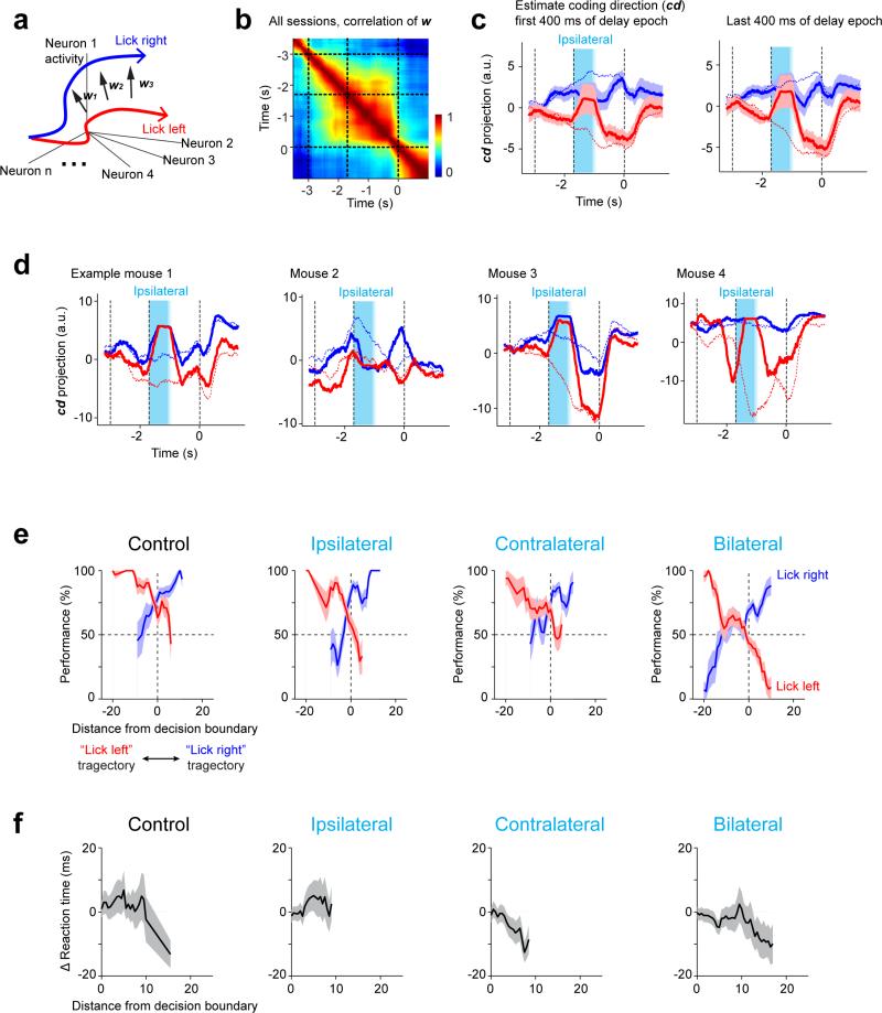
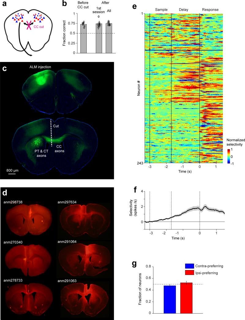
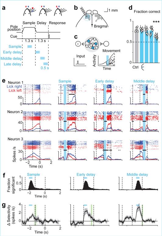
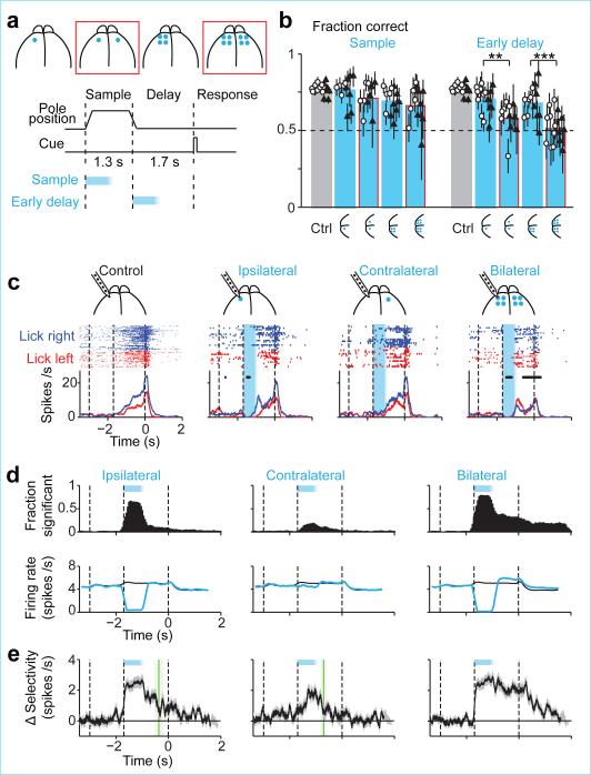
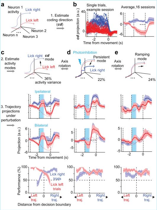
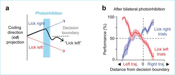
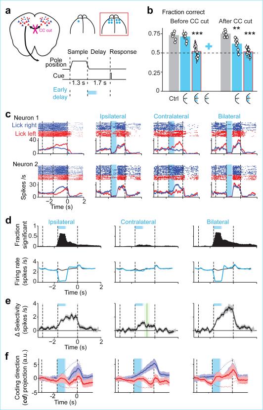
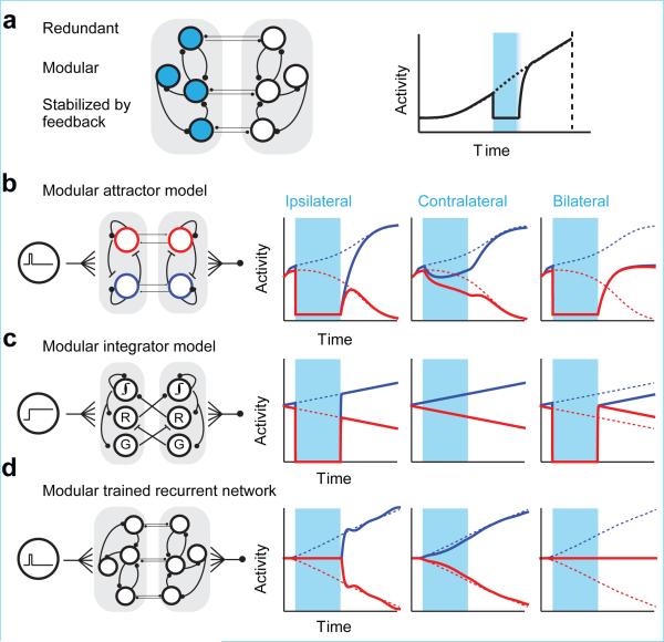
Neural activity maintains representations that bridge past and future events, often over many seconds. Network models can produce persistent and ramping activity, but the positive feedback that is critical for these slow dynamics can cause sensitivity to perturbations. Here we use electrophysiology and optogenetic perturbations in the mouse premotor cortex to probe the robustness of persistent neural representations during motor planning. We show that preparatory activity is remarkably robust to large-scale unilateral silencing: detailed neural dynamics that drive specific future movements were quickly and selectively restored by the network. Selectivity did not recover after bilateral silencing of the premotor cortex. Perturbations to one hemisphere are thus corrected by information from the other hemisphere. Corpus callosum bisections demonstrated that premotor cortex hemispheres can maintain preparatory activity independently. Redundancy across selectively coupled modules, as we observed in the premotor cortex, is a hallmark of robust control systems. Network models incorporating these principles show robustness that is consistent with data.

Extended Data Figure 1. Anterior lateral motor cortex (ALM) activity during motor planning and network models of premotor dynamics

a. Two example ALM neurons with selectivity during the object location discrimination task, out of 890 putative pyramidal neurons from 12 mice (Methods). Correct “lick right” (blue) and “lick left” (red) trials only. Dashed lines demarcate behavioral epochs. Averaging window, 200 ms. b. ALM population selectivity. Top panel, delay epoch was 1.3 s; bottom panel, delay epoch was 1.7 s. Selectivity is the difference in spike rate between the preferred and non-preferred trial type, normalized to the peak selectivity (Methods). Only putative pyramidal neurons with significant trial selectivity are shown (n=634/890). In addition, neurons tested for <15 trials for each trial type (19/634) were excluded. c. Average population selectivity in spike rate (black line, ± s.e.m. across neurons, bootstrap). d. Population response correlation. Pearson's correlation between the population response vectors at different times during the task and the population response vector at the onset of the ‘go’ cue (Time = 0). All selective putative pyramidal neurons were used, even if not recorded at the same time (ignoring potential correlations between neurons). To equalize the contributions of individual neurons, each neuron's response was mean-subtracted and normalized to the variance of its response across the entire trial (computed in time bins of 200 ms). e. Distribution of selectivity across the population during different epochs. For each neuron, a ROC value between “lick right” and “lick left” trials was computed using the spike counts during the particular behavioral epoch. Solid bars, neurons with significant trial-type selectivity (p<0.05, two-tailed t-test using spike counts). f-i, modeling description (reproduced from Methods) All networks were simulated for 2 seconds. Photoinhibition was simulated by holding the activity of half of the neurons in each network at zero for times 0.2 s < t < 1.0 s. Activity of the i^th neuron r_i(t) was governed by the equation: $$\tau \frac{d{r}_i\left(t\right)}{dt}=-r_i\left(t\right)+\sum _{j=1}^N{W}_{i,j}f\left(r_j\left(t\right)\right)+I_i\left(t\right)$$ where the cellular time constant τ, the connectivity matrix W and the synaptic non-linearity f(x) were chosen independently for each model. N is the number of neurons. In all simulations networks received either transient (0.05 s < t < 0.1 s) or persistent (0.1 s < t < 1.9 s) sensory inputs I_i(t) unless stated otherwise. The specifics of each model are described below. f. Simple integrator model. The network was simulated with N = 100 neurons, τ = 100 ms, and linear synapses (i.e. f (x) = x). The connectivity matrix was constructed so that all eigenvalues except for one were equal to zero. The non-zero eigenvalue was set to 0.99, producing feedback so that the firing rate of the network decays with a time constant given by τ / (1–0.99) =10s . In the network on the left the input was a task-selective persistent current I_i(t). In the simulation on the right the input was a task-selective transient input, and the signal from this integrator was then cascaded into a second identical network to produce ramping activity. Silencing was simulated by holding the activity of a randomly-selected population of 50 neurons at zero from times 0.2 s < t < 1.0 s. g. Integrator with corrective feedback. Corrective feedback is incorporated into an integrator network, consisting of a pair of excitatory and inhibitory neurons, to confer robustness against perturbations. This corrective feedback was achieved by a mismatch in the time constants for excitatory and inhibitory connections, which generates negative derivative feedback. The network exhibits robustness against random perturbations that equally affect the excitatory and inhibitory neurons, but is not robust against asymmetric activation of inhibitory neurons (e.g. photoinhibition). The function f(r) is determined by the differential equation : $${\tau }_{\mathrm{syn},i,j}\frac{d{f}_{i,j}\left(t\right)}{dt}=-f_{i,j}\left(t\right)+r_j\left(t\right).$$ The synaptic time constant τ_syn,i,j determines how quickly the post-synaptic currents respond to changes in presynaptic activity. The synaptic time constants were: inhibitory synapses, 10 ms; excitatory to inhibitory neurons, 25 ms; excitatory to excitatory neurons, 100 ms. As in the simple integrator model, the network received a task-selective persistent input. Photoinhibition was simulated by injecting large currents into the inhibitory neuron and disallowing negative firing rates, which results in silencing of the excitatory neuron. h. Randomly connected recurrent networks trained using FORCE learning to produce ramping dynamics (“trained RRNs”). FORCE learning is useful for training recurrent neural networks to produce custom input-output relationships that are relatively stable to noise. As stated in Methods: FORCE training was performed with τ = 200 ms, f(x) = tanh(x), N = 400. The network was given a brief pulse of external current during the interval 0.05 s < t < 0.1 s, representing transient sensory input. The initial connectivity matrix was chosen to be sparse with 90% of connections equal to zero. Non-zero connections were chosen from a Gaussian random distribution. The variance in connection strength was $\frac{{1.5}^2}{pN}$ where p=0.1 is the connection probability. 1.5 is a gain factor which is sufficiently strong to produce chaotic activity . Training was performed for 30 iterations where the weights were adjusted at each time step as described in . Each solid line represents the activity of the network's output in response to transiently clamping the activity of a randomly-selected population of 200 (i.e. N/2) neurons to zero. The network received either persistent (left) or transient (right) sensory input. For persistent input the network behaved similar to an integrator exhibiting a recovery of selectivity, albeit at an offset level upon removal of photoinhibition. i. RRN trained with FORCE as described above and further stabilized (tamed chaos). The algorithm was designed to stabilize selected trajectories in chaotic networks via a recursive retuning of recurrent connection strengths based on a recursive least-squares rule . To minimize the number of synapses that required tuning, the FORCE network was made sparse by eliminating weak connections that were smaller than an arbitrary threshold and using linear regression to slightly modify the remaining weights to maintain the dynamics. Elimination of weak synapses greatly reduced the time needed to train the network. Twenty iterations of the tamed chaos algorithm were then run with weights being adjusted every 10^th time step. Perturbations were applied as described for the FORCE trained network above. This training resulted in a modest increase in the robustness of the network.

Extended Data Figure 2. Characterization of photoinhibition

a. Silicon probe recording and photoinhibition in different experimental configurations used in this study. Experiment 1, data presented in Fig. 1, Extended Data Figs 3, 4; Experiment 2, data presented in Figs 2, 3, 4, Extended Data Figs 6, 8, 9; Experiment 3, data presented in Extended Data Fig. 7. b. Effect of photoinhibition on putative pyramidal neurons. For each neuron, spike rate during photoinhibition was normalized to spike rate in control trials. Left, experiment 1: n=117, 110, 109 neurons from 6 mice; experiment 2: n=300, 294, 301 from 7 mice; experiment 3: n=52, 52, 102 from 3 mice. Ipsilateral and bilateral photoinhibition similarly silenced neuronal activity. Average spike rate across the population was little affected by contralateral photoinhibition. Right, comparison of photoinhibition in VGAT-ChR2-EYFP mice and PV-ires-cre mice crossed to a ReaChR reporter line (Methods) . Photoinhibition was similar in the two mouse lines (>90% activity reduction). Data from ipsilateral photoihibition from experiment 2 (n=94 neurons from 3 VGAT mice; n=201 from 4 PV-cre × ReaChR mice). Error bars, s.e.m. over neurons. Neurons with mean spike rate of <1 spikes/s were excluded. c. Top, photostimuli were shaped to minimize rebound activity after photoinhibition. Peak photostimulus intensity was gradually reduced over 200 ms during stimulus offset. Bottom, average spike rate across the population (black, control; cyan, photoinhibition). Data from experiment 2, ipsilateral photoinhibition, n=300 neurons from 7 mice. d. Effect of photoinhibition versus distance from the laser center under the standard photostimulus (1 laser spot). Neurons were pooled across cortical depths. Recording data were obtained from ALM of 4 untrained mice under awake and non-behaving conditions. Recording procedures were described in . Thin lines, individual mice (n=246 neurons, 2 VGAT-ChR2-EYFP mice, 2 PV-ires-cre × ReaChR mice). e. Average spike rates on control versus photoinhibition “lick right” trials during different epochs of the task. Data from experiment 2. Photoinhibition was for 800ms at the beginning of the delay epoch. The delay epoch was 1.7s. Columns from left to right: the last 400ms of the sample epoch, the first 400ms of the photoinhibition, the last 400ms of the photoinhibition, the first 400ms after photoinhibition, 400-800ms after photoinhibition, first 400ms of the response epoch (see a for trial structure). Top row, ipsilateral photoinhibition (1 laser spot, Methods); middle, contralateral photoinhibition (1 laser spot); bottom, bilateral photoinhibition (4 laser spots). Colored dots, neurons with significant spike rate change (p<0.01, two tailed t-test). Crosses, population means. No rebound excitation was detected after photoinhibition offset on average (d). A small proportion of neurons showed rebound excitation which was balanced by a low level of sustained inhibition in a larger proportion of neurons. Results are similar for “lick left” trials (not shown).

Extended Data Figure 3. Unilateral photoinhibition of ALM immediately before movement causes ipsilateral bias

a. Unilateral photoinhibition of ALM during different task epochs. Sample epoch, 1.3s; delay epoch, 1.3s. Photoinhibition, 0.5 s (0.4s and 0.1s ramp, Methods). b. Performance with 0.5s photoinhibition of left or right ALM during different trial epochs. Performance was plotted as a function of time interval between photoinhibition offset (the end of ramp offset) and the onset of ‘go’ cue (T_recovery). Performance was not significantly affected for T_recovery>0.3s. Thick lines, mean; thin lines, individual mice (n = 5). *p<0.05, **p<0.01, ***p < 0.001, two-tailed t-test. c. Unilateral photoinhibition of ALM during different task epochs. Sample epoch, 1.3s; delay epoch, variable duration, 1.2s – 1.7s in 0.1s increments. Trials with different delay epoch durations were randomly interleaved. Photoinhibition was for 1.3s (1.2s and 0.1s ramp, Methods), resulting in different T_recovery. d. Performance with 1.3s photoinhibition. Plot is similar to (b). Performance was not significantly affected for T_recovery > 0.3s. e. Photoinhibition (0.5 s) immediately before the ‘go’ cue is similar to the behavioral effect caused by photoinhibition during the entire delay epoch (1.3 s). Photoinhibition data at T_recovery=0 from (b) and (d) was re-plotted.

Extended Data Figure 4. ALM neurons with decreasing spike rates during the delay epoch recovered their normal spike rates after unilateral photoinhibition

a. Three example ALM neurons with decreasing spike rates during the delay epoch. Top, spike raster. Bottom, PSTH. All “lick right” (blue) and “lick left” (red) trials. Dashed lines, behavioral epochs. Blue shades, photoinhibition. b. Normalized spike rate for all neurons with significant spike rate decrease at the end of the delay epoch compared to the beginning of the delay epoch (p < 0.05, two-tailed t-test; 400 ms windows; pooled across trial types). 27 neurons from 6 mice. The spike rate for each neuron was normalized to the mean spike rate. Blue, preferred trial type; red, non-preferred. Mean ± s.e.m. across neurons, bootstrap. Dotted lines, spike rates in control trials. c. The data is consistent with a return to the normal trajectory and inconsistent with decay to the end point. Top, spike rate difference between perturbed trials and the time-matched spike rates in control trials. Bottom, spike rate difference between perturbed trials and the spike rates at the end of the delay epoch in control trials. Data from (b). Mean ± s.e.m. across neurons, bootstrap. Spike rate difference relative to time-matched control show significantly smaller root-mean-squared error (RMS) than spike rate difference relative to end point (p<0.001, paired t-test). RMS was computed during the epoch between photoinhibition offset and the ‘go’ cue.

Extended Data Figure 5. Preparatory activity is robust to photoactivation

a. Left, silicon probe recording during unilateral photoactivation of a subset of excitatory neurons. Tlx_PL56-Cre mice (MMRRC 036547) were crossed to Ai32 (Rosa26-ChR2 reporter mice, JAX Stock#012569) to express ChR2 in layer 5 intratelencephalic (IT) neurons . Right, task structure and timing of photoactivation (cyan). b. Top, photostimulus. Bottom, average spike rate across the population (n = 69 neurons from 2 mice). Black, control; cyan, photoactivation. Rebound inhibition was observed after photoactivation. c. Effect of photoactivation on spike rates. Data is for photoactivation during early delay epoch. Black circles, neurons with significant spike rate change (p<0.01, two tailed t-test). Photoactivation during sample epoch: 19% excited, 22% suppressed; late delay epoch: 15% excited, 17% suppressed. “Lick right” and “lick left” trials were pooled to compute spike rates. d. Three example ALM neurons. Top, spike raster. Bottom, PSTH. All “lick right” (blue) and “lick left” (red) trials. Dashed lines, behavioral epochs. Blue shades, photoinhibition. e. Top, significant spike rate changes relative to control are highlighted for individual neurons. Neurons (rows) are sorted based on their mean spike rate across the trial epoches. Neurons with mean spike rate below 1 spikes/s or tested for less than 3 trials are excluded. Middle, fraction of neurons with significant spike rate change (n=43, 44 from 2 mice). Bottom, average spike rate across the population. f. Average population selectivity change from control (ΔSelectivity ± s.e.m. across neurons, bootstrap). Only selective neurons tested for >3 trials in all conditions are shown (n=26). Green lines, time points when the selectivity recovered to 80% of control selectivity (mean ± s.e.m. across neurons, bootstrap). Sample epoch: 249 ± 68 ms to recover to 80 % of control selectivity; early delay: 275 ± 168 ms; middle delay: 250 ± 218 ms.

Extended Data Figure 6. ALM dynamics predicts upcoming movements at the level of behavioral sessions

a. Behavioral performance on control and bilateral photoinhibition trials. b. Time course of activity trajectories projected onto the coding direction (cd). Dotted lines, average trajectories from control “lick right” (blue) and “lick left” (red) trials. Solid lines, average trajectories from bilateral photoinhibition trials. Each plot shows data from one session for one mouse. Trajectories in photoinhibition trials were similar to control trials before photoinhibition and were persistently altered by transient bilateral photoinhibition. The resultant trajectories were inconsistent from session to session: in some cases the altered trajectories were closer to the “lick right” control trajectories (blue dotted lines), and in other cases closer to the “lick left” control trajectories (red dotted lines). Averaging window, 400ms. In sessions with altered activity trajectories that were closer to the control “lick left” trajectories, movements were biased to the left, resulting in high performance in “lick left” trials and low performance in “lick right” trials (session 1, 4). The opposite behavioral bias was observed when altered activity trajectories were closer to the control “lick right” trajectories (session 2, 3, 5). The biases in movement were predicted based ALM activity trajectories. Session 1-5, n=20, 16, 18, 10, 12 neurons.

Extended Data Figure 7. Bilateral photoinhibition disrupts ALM dynamics and behavior

a. Silicon probe recording during unilateral (4 laser spots) and bilateral (1 laser spot; red box) photoinhibition. b. Behavioral performance. Bar, mean across all mice (n=3). Symbols, individual mice (mean ± s.e.m, bootstrap). c. Top, significant spike rate changes for individual neurons (black). Neurons (rows) are sorted based on their mean spike rate across the trial epoches. Neurons with mean spike rate below 1 spikes/s or tested for less than 3 trials are excluded (n=60, 59, 60). Photoinhibition is indicated on the top. Bottom, fraction of neurons with significant spike rate change. d. Average population selectivity change from control (ΔSelectivity ±s.e.m. across neurons, bootstrap). Only selective neurons tested for >3 trials in all conditions are shown (n=40). Green lines, time points when the selectivity recovered to 80% of control selectivity (mean ± s.e.m. across neurons, bootstrap). Ipsilateral: 490±280 ms to recover to 80% of control selectivity; contralateral: 235±156 ms; bilateral: no recovery at end of delay period. e. Time course of activity trajectories on “lick right” (blue) and “lick left” (red) trials projected onto the coding direction (cd). Average trajectories from all sessions (± s.e.m. across sessions, bootstrap, Methods). From left to right panels: control trials, ipsilateral photoinhibition (4 laser spots), contralateral photoinhibition (4 laser spots), and bilateral photoinhibition (1 laser spot). Dotted line, trajectories in control trials. Only sessions with >5 simultaneously recorded neurons tested for >3 trials in each condition. We quantified the separation between trajectories at the end of delay epoch by computing ROC values for each session: control, 0.80 ± 0.08; ipsilateral, 0.64 ± 0.10; contralateral, 0.68 ± 0.15; bilateral, 0.54 ± 0.8. Mean ± s.e.m. across sessions, Methods.

Extended Data Figure 8. Decomposition of ALM dynamics after perturbation

a. Decomposition of activity into five modes based on control trials and ipsilateral perturbations (Methods). Fraction of activity variance (left) and selectivity (right) explained by modes 1-5. The overlap in variance and selectivity between mode 1 and modes 2 & 3 are highlighted in black. Error bars, s.e.m. across sessions. Data from 16 sessions, 7 mice. Activity variance here is computed using trial-averaged activity (Methods), thus they reflect variance across time and neurons. Activity variance across trials is not reflected. The fraction of variance explained for the single-trial activity would be much lower. b. Fraction of upcoming movements predicted based on modes 1-5. Trajectory distance from the decision boundary at the time of the ‘go’ cue is used to predict behavior. “Lick right” and “lick left” trials are pooled. Error bars, s.e.m. across sessions. c. Projections of activity along modes 1-5 for ipsilateral perturbation trials (solid). Dashed blue and red lines correspond to the means for control trials. Errorbars, s.e.m. across sessions. For the cd mode, a different set of trials was used here to compute cd compared to Fig. 3c (Methods). This resulted in small differences in the projected trajectories. d. Projections of activity in the same dimensions as in (c) for contralateral perturbation trials. e. Projections of activity in the same dimensions as in (c) for bilateral perturbation trials. f. Weights of each neuron for mode 1 versus modes 2-5. Mode 1 and modes 2-5 involve overlapping populations of neurons. Data from all sessions were pooled. Note that the ramping modes (4 & 5) are resistant to all perturbations, including bilateral perturbations, suggesting that overall ramping may be driven by a source external to ALM. ROC values between trajectories along the cd mode at the end of delay epoch: control, 0.76 ± 0.03; ipsilateral, 0.73 ± 0.02; contralateral, 0.74 ± 0.03; bilateral 0.58 ± 0.03. ROC values during the time period of photoinhibition: control, 0.72 ± 0.02; ipsilateral, 0.54 ± 0.03; contralateral, 0.64 ± 0.03; bilateral 0.54 ± 0.01.

Extended Data Figure 9. ALM dynamics along the coding direction predicts upcoming movements

a. Schematic of trajectory analysis in activity space. The difference in the mean response vectors between “lick right” and “lick left” trials, w, was estimated across different time windows (400ms) during sample and delay epochs. b. w are similar during sample and delay epoch. Correlation of w's across time. Data from 16 sessions, 7 mice. The coding direction, cd, was taken as the average of w over time. c. The recovery of ALM dynamics along the coding direction (cd) is robust to the choice of time window for the calculation of cd. Left, cd was the average of w's from the first 400 ms of the delay epoch. Right, cd was the average of w's from the last 400 ms of the delay epoch. d. The recovery of ALM dynamics along cd is robust across mice. e. Behavioral performance in “lick right” and “lick left” trials as a function of trajectory distance from the decision boundary at the time of the ‘go’ cue. Positive values on the x-axis indicate closer distance to the control “lick right” trajectory. From left to right panels: control trials, ipsilateral photoinhibition trials, contralateral photoinhibition trials, and bilateral photoinhibition trials. Performance was computed by binning along the cd distance (bin size, 4 on the cd distance scale). s.e.m. was obtained by bootstrapping the trials in each bin. f. Reaction times are faster on trials in which the trajectory is far from the decision boundary at the time of the ‘go’ cue. ΔReaction time is relative to the mean reaction time from each session. Data from 16 sessions, 7 mice. Data from “lick right” and “lick left” trials were pooled.

Extended Data Figure 10. Behavioral and ALM dynamics after Corpus Callossum (CC) hemisection

a. Schematic. CC was bisected while sparing the pyramidal tract (PT) and corticothalamic (CT) projections. b. Behavioral performance. Bar, mean across all mice (n=7). Symbols, individual mice (mean ± s.e.m, bootstrap). Performance was not affected by the CC bisection. 1^st session was ~ 17 hours after the CC bisection. c. Location of the CC cut superimposed on axonal projections from ALM. AAV2/1-CAG-EGFP was injected into ALM. A vertical cut ~3.5 mm deep was made approximately 0.5 mm from the mid-line. The cut extended from bregma anterior 1.5 mm to posterior 1 mm. The cut was either made in the left hemisphere (3 mice) or the right hemisphere (4 mice). The cut spared the PT and CT axons. d. Coronal section showing the CC bisection in 6 mice. Left column, autofluoresence; right column, GFAP immunofluorescence (Methods). e. ALM shows normal preparatory activity after the CC bisection. ALM population selectivity. Selectivity is the difference in spike rate between the preferred and non-preferred trial type, normalized to the peak selectivity (Methods). Only putative pyramidal neurons with significant trial selectivity are shown (n=254/496). In addition, 11/254 neurons tested for <15 trials for each trial type were excluded. f. Average population selectivity in spike rate (black line, ± s.e.m. across neurons, bootstrap). g. Proportion of contra-preferring vs. ipsi-preferring neurons. Error bars, s.e.m. across mice, bootstrap.

Figure 1. ALM preparatory activity is robust to photoinhibition

a. Mice discriminate pole location during the sample epoch and respond “lick right” or “lick left” after a delay. Cyan, photoinhibition. b. Grey, ALM; area that produced behavioral effects with photoinhibition throughout the delay epoch (Methods; Allen Reference Atlas). Cyan, contours of photoinhibition (small, 90% reduction in activity; medium, 80%; large/dashed, 50%). c. Schematic network models and responses to transient inactivation of subsets of neurons (cyan). Dashed line, unperturbed activity trajectory; solid line, perturbed activity trajectories. d. Behavioral performance (see timing in a). Bar, mean. Symbols, individual mice (mean ± s.e.m, bootstrap). ***p<0.001, two-tailed t-test against control. e. Example neurons. Top, spike raster. Bottom, PSTH, averaged over 200 ms. “Lick right” (blue) and “lick left” (red) trials, grouped by instructed movement. Dashed lines, behavioral epochs. Cyan, photoinhibition. Black ticks above PSTH, significant spike rate change (p<0.01, two-tailed t-test). f. Fraction of neurons with significant spike rate change (n=168, 168, 175). Cyan, photoinhibition. g. ΔSelectivity from control (mean ± s.e.m. across neurons, bootstrap; selective neurons tested for >3 trials in all conditions, n=55). Green lines, recovery to 80% of control (mean ± s.e.m. bootstrap). Sample, 373±260 ms; early delay, 510±218 ms; late delay, 327±112 ms.

Figure 2. Bilateral photoinhibition disrupts preparatory activity

a. Unilateral and bilateral (red) photoinhibition. b. Behavioral performance. Bar, mean. Symbols, individual mice (mean ± s.e.m, bootstrap). Open circle, photoinhibition duration, 800 ms; solid triangle, 1300 ms. **,p<0.01, ***, p<0.001, two-tailed t-test against control. c. Example ALM neuron. Cyan, photoinhibition. d. Fraction of neurons with significant spike rate change (n=276, 283, 332). Bottom, average spike rate across the population (black, control; cyan, photoinhibition). e. Average change in population selectivity from control (n=143). Same as Fig. 1g. Selectivity recovery: ipsilateral, 538±178 ms; contralateral, 192±114 ms; bilateral, no recovery.

Figure 3. Preparatory activity preferentially recovers along coding dimension in activity space

a. Schematic, movement-specific trajectories in activity space. b. Left, activity on correct “lick right” (blue) and “lick left” (red) trials projected onto the coding direction (cd). One session, 12 neurons. Right, average trajectories from all sessions (± s.e.m. bootstrap, Methods). All unperturbed trials (correct and incorrect), grouped by instructed movement. Dotted gray line, decision boundary. Averaging window, 400 ms. c. Top, illustration of the cd mode. Middle, activity in ipsilateral and bilateral photoinhibition trials projected onto the cd. All perturbed trials (correct and incorrect), grouped by instructed movement. Dashed blue and red lines, means for unperturbed trials (from b). Bottom, behavioral performance in “lick right” (blue) and “lick left” (red) trials as a function of trajectory distance from the decision boundary. Performance was computed by binning along the cd distance. s.e.m. was obtained by bootstrapping the trials in each bin. d. Same as (c) for activity along persistent mode, which maximizes the difference between perturbed and unperturbed activity at the time of movement onset. This mode does not carry movement-specific information (middle; note that red and blue dashed lines are near each other) and does not predict movement direction (bottom). e. Same as (c) for population activity along the ramping mode, which explains most of the remaining activity variance (Methods). This mode shows robust ramping but is non-selective (middle) and does not predict movement direction (bottom).

Figure 4. ALM predicts upcoming movements after bilateral perturbations

a. Schematic, using preparatory activity projected onto the coding direction (cd) to predict upcoming movement. b. Behavioral performance as a function of trajectory distance from the decision boundary. Same as Fig. 3c for bilateral photoinhibition trials. See Extended Data Fig. 9 for unilateral photoinhibition trials.

Figure 5. Contralateral ALM input is required for recovery of preparatory activity

a. Left, corpus callosum (CC) bisection. Right, unilateral and bilateral photoinhibition during early delay epochs. b. Behavioral performance. Bars, mean. Symbols, individual mice (mean ± s.e.m, bootstrap). **,p<0.01, ***, p<0.001, two-tailed t-test against control. Cyan cross, performance for bilateral photoinhibition, 1 spot, in a separate group of control mice (data from Fig. 2b). c. Two example ALM neurons, after callosotomy. d. Fraction of neurons with significant spike rate change (n=325, 322, 313). Bottom, average spike rate across the population. e. Average change in population selectivity from control (n=129). Same as Fig. 2e. Selectivity recovery: ipsilateral, no recovery; contralateral, 217±228 ms; bilateral, no recovery. f. Population activity in photoinhibition trials projected onto the coding direction (cd). Same as Fig. 3c for ipsilateral, contralateral, and bilateral photoinhibition.

Figure 6. Modular network models of premotor dynamics

a. Schematic, a modular network robust to transient inactivation of one module. b. Modular attractor model. Neurons with right (blue) and left (red) preferences provide self-excitation and mutual inhibition. Connections between modules involve neurons with similar preference. See Methods for model parameters in b-d. c. Modular integrator model . Connections between modules restore activity on other side (“recovery” neurons, “R”). Gating neurons (labeled “G”) cancel the inter-module coupling during normal operation. d. Modular recurrent network trained with FORCE learning to recapitulate single hemisphere perturbation.

References

1. Tanji J, Evarts EV. Anticipatory activity of motor cortex neurons in relation to direction of an intended movement. J Neurophysiol. 1976;39:1062–1068. - PubMed
1. Churchland MM, Cunningham JP, Kaufman MT, Ryu SI, Shenoy KV. Cortical preparatory activity: representation of movement or first cog in a dynamical machine? Neuron. 2010;68:387–400. - PMC - PubMed
1. Guo ZV, et al. Flow of cortical activity underlying a tactile decision in mice. Neuron. 2014;81:179–194. - PMC - PubMed
1. Erlich JC, Bialek M, Brody CD. A cortical substrate for memory-guided orienting in the rat. Neuron. 2011;72:330–343. - PMC - PubMed
1. Murakami M, Vicente MI, Costa GM, Mainen ZF. Neural antecedents of self-initiated actions in secondary motor cortex. Nature neuroscience. 2014;17:1574–1582. - PubMed
Publication types