Primary motor and sensory cortical areas communicate via spatiotemporally coordinated networks at multiple frequencies

Abstract

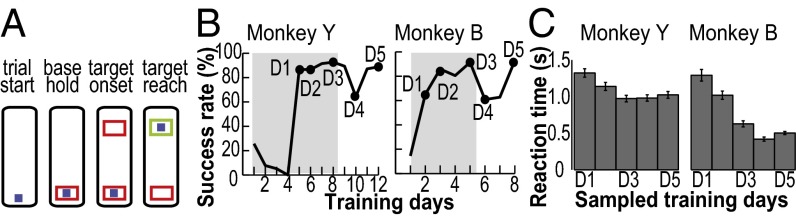
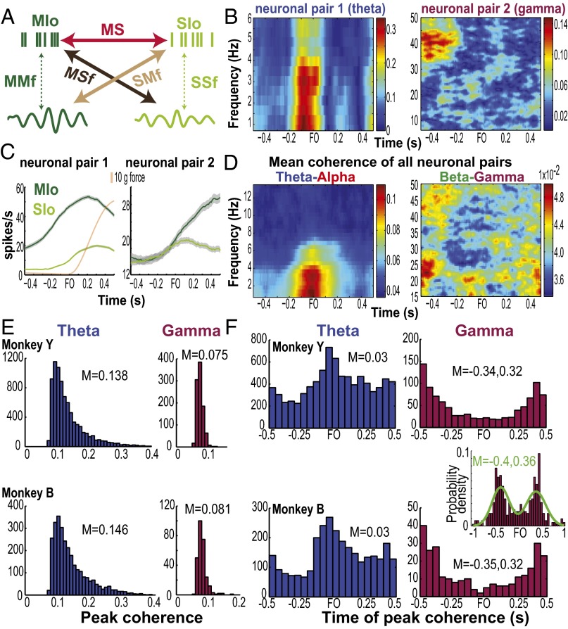
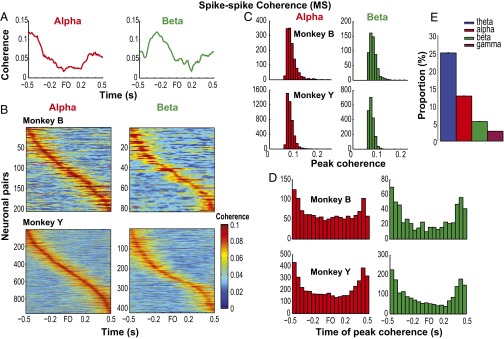
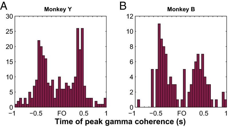
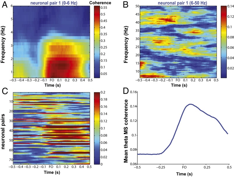
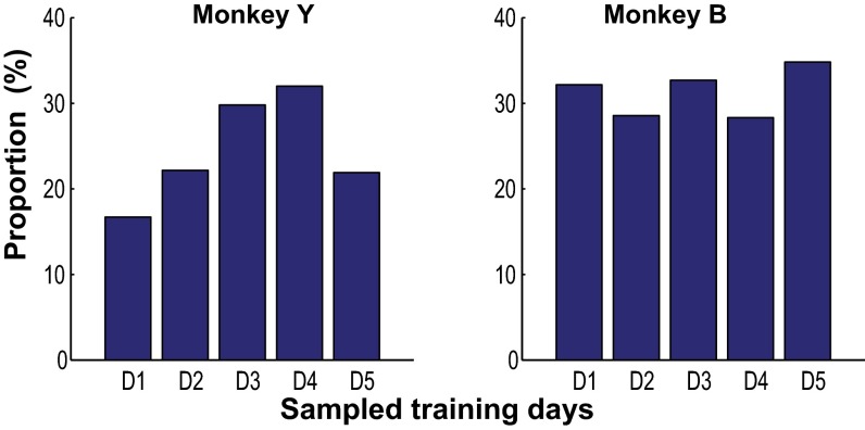
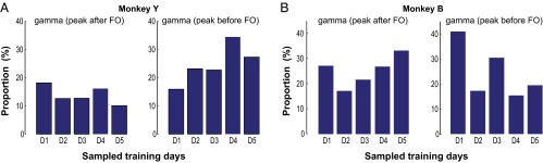
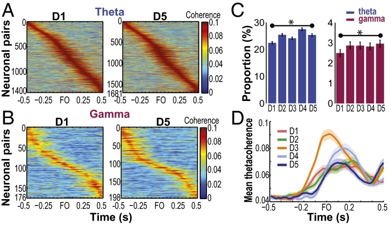
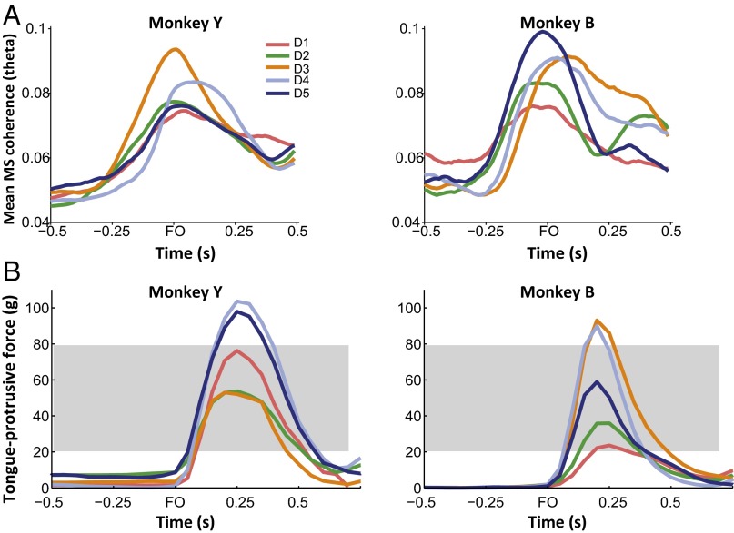
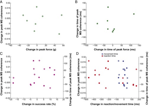
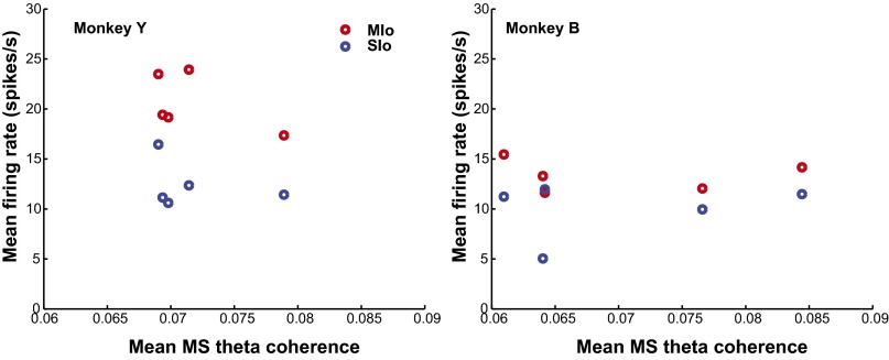
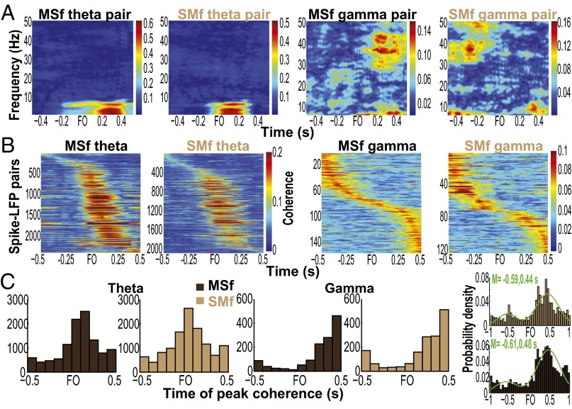
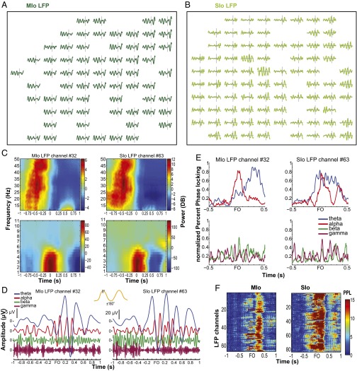
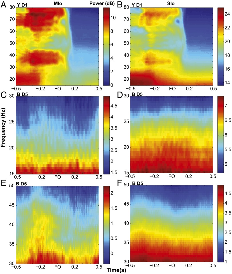
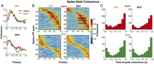
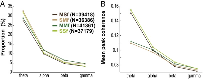
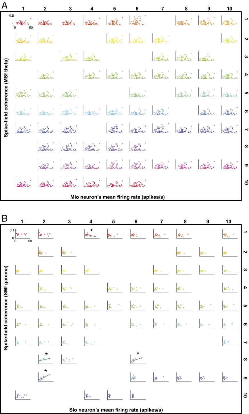
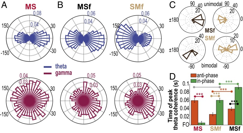
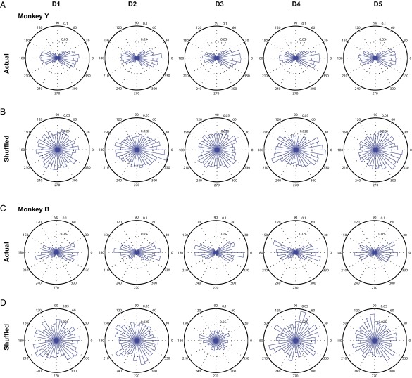
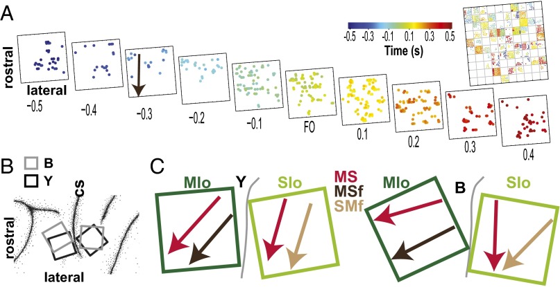
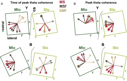
Skilled movements rely on sensory information to shape optimal motor responses, for which the sensory and motor cortical areas are critical. How these areas interact to mediate sensorimotor integration is largely unknown. Here, we measure intercortical coherence between the orofacial motor (MIo) and somatosensory (SIo) areas of cortex as monkeys learn to generate tongue-protrusive force. We report that coherence between MIo and SIo is reciprocal and that neuroplastic changes in coherence gradually emerge over a few days. These functional networks of coherent spiking and local field potentials exhibit frequency-specific spatiotemporal properties. During force generation, theta coherence (2-6 Hz) is prominent and exhibited by numerous paired signals; before or after force generation, coherence is evident in alpha (6-13 Hz), beta (15-30 Hz), and gamma (30-50 Hz) bands, but the functional networks are smaller and weaker. Unlike coherence in the higher frequency bands, the distribution of the phase at peak theta coherence is bimodal with peaks near 0° and ±180°, suggesting that communication between somatosensory and motor areas is coordinated temporally by the phase of theta coherence. Time-sensitive sensorimotor integration and plasticity may rely on coherence of local and large-scale functional networks for cortical processes to operate at multiple temporal and spatial scales.

Keywords: coherence; learning; motor cortex; orofacial cortex; somatosensory cortex.

Fig. 1.

Behavioral task and performance. (A) Diagram of the sequence of events in a trial of the tongue protrusion task. The blue square represents the force cursor, whereas the red and green boxes represent the base and force targets. (B) Success rates shown separately for each monkey. Dots mark the 5 d that were analyzed (i.e., sampled training days D1 to D5). Shaded area corresponds to training days when the required force level was 50 g. Required force level was increased to 80 g when success rates reached >75% for at least 3 consecutive days. (C) Reaction time shown as mean (±1 SEM error bars) across all trials for D1 to D5. B and C adapted from ref. .

Fig. 2.

Frequency-specific modulation of MS coherence between MIo and SIo neurons. (A) Schema of paired signals used in interareal coherence: paired spikes from MIo and SIo (MS), paired MIo spikes and SIo LFPs (MSf), and paired SIo spikes and MIo LFPs (SMf). We also analyzed intraareal coherence, i.e., paired spikes and LFPs within each area (MMf and SSf). (B) Coherogram of two pairs of neurons with significant MS coherence (color scale). Coherence is aligned to the right edge of the 0.5-s window, e.g., coherence at force onset (FO) corresponds to a 0.5-s window ending at FO. (C) Mean firing rates of MIo and SIo neurons whose coherent activity is shown in B. Rates were calculated using a 0.5-s sliding window with 0.01-s steps per trial then averaged across trials. Gray shades denote 1 SEM. Orange line denotes mean tongue-protrusive force of the first 100 trials of a training day. The force profile is averaged over a 0.5-s window. Timescales for rates and force are plotted to the right edge of 0.5-s window over which they were computed. (D) Mean coherence across all unique pairs of neurons (SI Methods) with significant coherence in one dataset, shown for the theta–alpha bands (n = 75 pairs) and beta–gamma bands (n = 67), respectively. (E) Histograms of peak coherence of all pairs with significant coherence in the theta and gamma bands. Shown for monkeys Y (n_theta = 8,148, n_gamma = 967) and B (n_theta = 2,874, n_gamma = 271) separately. Data pooled across D1 to D5. M, mean. (F) As in E, for time of peak coherence. (Inset) Histogram of time of peak gamma coherence ranging from –1.5 and 1 s relative to FO. Green line indicates Gaussian mixture model fit using two components. Data include only unique neuronal pairs with significant modulation of coherence, pooled across days and monkeys.

Fig. S1.

Modulation of spike–spike coherence (MS) in the alpha and beta bands. (A) Spike–spike coherence (MS) of a pair of neurons in the alpha and beta bands. (B) MS coherence of neuronal pairs (rows) that showed significant task modulation of coherence in the alpha (Left) and beta (Right) bands. Color represents the magnitude of coherence, and the neuronal pairs were sorted according to the time of peak coherence relative to FO. Shown for one dataset (D3) from each monkey (rows). (C and D) Histograms of peak MS coherence and time of peak MS coherence, respectively, in the alpha and beta bands. Shown for monkeys Y and B separately. (E) Proportion of neuronal pairs with significant modulation of MS coherence in each frequency band. Data pooled across all training days and monkeys (n_theta = 11,022, n_alpha = 5,632, n_beta = 2,444, n_gamma = 1,238).

Fig. S2.

Suppression of MS gamma coherence around force onset. (A and B) Distributions of time of peak MS coherence in the gamma band shown for monkeys Y and B, respectively. By extending the time windows analyzed relative to FO, each distribution shows peaks around ±0.5 s relative to FO. Data pooled across training days but include only unique neuronal pairs (SI Methods) for each training day.

Fig. S3.

Coherence using 1-s time window. (A and B) Coherograms show the MS coherence of a neuronal pair as a function of time (x axis, using a 1-s time window) and frequency (y axis) in the 0- to 6-Hz and 6- to 50-Hz ranges, respectively. (C) MS theta coherence of nonoverlapping (unique) neuronal pairs recorded from D3. (D) Mean MS theta coherence across the neuronal pairs shown in C. Note that the time of peak coherence in the 1-s window was comparable to a 0.5-s window.

Fig. S4.

Cross-validation of time of peak MS coherence in the theta band. Proportion of neuronal pairs in the test subset with significant MS coherence at the mean time of peak MS coherence determined by the training subset of neuronal pairs. Shown for each sampled training day D1 to D5 for monkeys Y and B.

Fig. S5.

Cross-validation of time of peak MS coherence in the gamma band. (A and B) Proportion of neuronal pairs in the test subset with significant MS coherence at the mean time of peak MS coherence determined by the training subset of neuronal pairs shown for monkeys Y and B, respectively. Cross-validation test was performed on two peak times corresponding to the means based on a two-component Gaussian mixture model fit.

Fig. 3.

Modulation of MS coherence by learning. (A and B) MS coherence of neuronal pairs with significant coherence in the theta and gamma bands, respectively, for D1 and D5 of monkey Y. Each plot shows changes in coherence of a neuronal pair (corresponding to a row in the y axis) relative to FO. Neuronal pairs are sorted according to the time of peak coherence relative to FO. (C) Day-to-day changes in the proportion of neuronal pairs with significant modulation of MS coherence. Data pooled across monkeys: in both theta and gamma bands, proportion increased from D1 (n_theta = 1,971/8,770, n_gamma = 219/8,770) to D5 (n_theta = 2,306/9,089, n_gamma = 269/9,089). *P < 0.05. Error bars indicate ±1 SEM (based on a binomial distribution assumption). (D) Day-to-day changes in MS theta coherence. Shown as mean (±1 SEM) coherence across pairs of stable neurons in monkey Y.

Fig. S6.

Day-to-day changes in MS coherence cannot be explained by changes in tongue-protrusive force. (A) Mean MS coherence across neuronal pairs that showed significant coherence in the theta band. Shown for each training day of monkeys Y and B. The change of peak MS coherence relative to D1 [e.g., delta = (D2 peak – D1 peak)/D1 peak] ranged from 2% to 26% in monkey Y and 9% to 30% in monkey B. (B) Mean tongue-protrusive force across the first 100 successful trials for the corresponding days in A. Shaded gray area corresponds to the force target window for the 50-g target set for D1–D3. On D1, monkey B was learning to gauge how much force was needed. On D2, success rates increased indicating that the monkey was applying more force than he did on D1. Monkey used the same strategy on D3, suggesting that the monkey might have associated increased success rates with increased force. In principle, the monkey could have used a strategy in which he applied maximal force because he was not required to hold the force at the target. However, in practice, that was not observed. In monkey Y, the peak tongue force on D1–D3 never exceeded the upper boundary of the gray area. This was also true for D1–D2 in monkey B. Both monkeys did not exceed the upper force boundary (110 g) for D4–D5.

Fig. S7.

Changes in MS theta coherence were not correlated with changes in behavior. (A) Correlation between day-to-day changes in peak force and changes in peak MS theta coherence. Day-to-day change was calculated as the difference between the mean values of two consecutive days (n = 8, 4 data points per monkey). (B) As in A, for correlation between time of peak force and time of peak MS theta coherence. (C) Correlations of changes in success rate and changes in peak MS theta coherence (empty circles) and time of peak MS theta coherence (filled circles) were not significant (Pearson’s correlation, P > 0.10). (D) As in C, for reaction and movement times (Pearson’s correlation, P > 0.10).

Fig. S8.

Changes in MS theta coherence across training sessions do not follow mean firing rates of MIo and SIo neurons. Scatterplot of mean firing rates (across all MIo or SIo neurons) of each sampled training day (D1–D5) and the mean MS theta coherence across all pairs for the time window –0.3–0.2 s relative to FO, shown for each monkey. No significant correlation was found between mean firing rates and mean MS theta coherence (Pearson’s correlation, P > 0.10 for each monkey and for each cortical area). Similar results were found with other time windows (from 0.5 s before FO until FO, from FO to 0.5 s after FO).

Fig. 4.

Network-specific modulation of spike–field coherence. (A) Each coherogram shows spike–field coherence (MSf or SMf) of a single pair of signals as a function of frequency. (B) Theta and gamma spike–field coherence (MSf or SMf) of a population of pairs (y axis) from one dataset. Each row is a coherogram from a pair of signals and is the average over the theta (2–6 Hz) or gamma (30–50 Hz) band. Paired signals are sorted according to the time of peak coherence relative to FO. (C) Histograms of time of peak coherence for theta and gamma bands in MSf and SMf. Data pooled across training days and monkeys. (Inset) Histograms of time of peak gamma coherence (SMf and MSf) ranging from –1.5 and 1 s relative to FO. Green line indicates Gaussian mixture best model fit using two components. M, mean.

Fig. S9.

Rhythmic oscillations in the primate orofacial sensorimotor cortex. (A) Single-trial LFPs from MIo or SIo. Each subplot illustrates bandpass-filtered (2–6 Hz), single-trial LFPs recorded from one electrode of the microelectrode array implanted in MIo. Horizontal gray lines in each subplot denote 0 μV and time window from 1 s before force onset to 0.5 s after force onset (FO). Vertical gray lines in each subplot denote ±50-μV LFP amplitude and force onset. Data from training day 3 of monkey Y. (B) As in A, for SIo LFPs, except that vertical gray lines denote ±225-μV LFP amplitude. (C) Trial-averaged spectrograms of LFPs from a single channel in MIo and in SIo. We used a 0.5-s sliding window with 0.01-s steps to calculate the power spectrum. We then subtracted the mean power (per frequency for ±1 s relative to FO) from the power at each time point and frequency. Different scales for spectral power were used for 1–11 Hz and 11–50 Hz to show the modulation of power in the low versus high frequencies. (D) Bandpass-filtered trial-averaged LFPs from the same channels shown in C, aligned to FO, and plotted relative to 0 μV. Inset waveform shows peak and trough of the oscillation corresponds to 0° and ±180°, respectively. (E) Normalized percent phase locking (PPL) as a function of time for MIo and SIo channels shown in C. Shown for each frequency band. (F) Theta band’s PPL relative to FO (represented by color scale). Shown for all LFP channels in MIo (Top) and in SIo (Bottom). Each row of a subplot corresponds to one LFP channel.

Fig. S10.

Modulation of spectral power in MIo and SIo do not follow the modulation of coherence. (A and B) Spectrograms of mean power across all LFPs in MIo and SIo from D1 of monkey Y. Spectral power of beta (15–30 Hz) in MIo and SIo was high before FO. Attenuation of beta power occurred around 0.2 s before FO and was sustained until 0.5 after FO. The modulation of gamma power (30–50 Hz) in MIo and SIo was different from that of gamma coherence; gamma power was high before FO until 0.1 s after FO when it decreased and remained low until 0.5 s after force onset. (C–F) As in A and B, for D5 of monkey B. Different power scales were used for beta (C and D) and gamma (E and F). No attenuation of beta power was found in MIo nor SIo. Modulation of gamma power was evident in MIo but not in SIo.

Fig. S11.

Modulation of spike–field coherence in the alpha and beta bands. (A) Spike–field coherence of a paired signal in SMf and another in MSf in the alpha and beta bands. (B) Spike–field coherence of neuronal pairs (rows) that showed significant task modulation of coherence in the alpha (Top) and beta (Bottom) bands. Color represents the magnitude of coherence, and the spike–LFP pairs were sorted according to the time of peak coherence relative to FO. Shown for SMf (left column) and MSf (right column). Data from D5 of monkey Y. (C) Histograms of time of peak coherence for alpha and beta bands in SMf and MSf. Data pooled across sampled training days and monkeys.

Fig. S12.

Properties of spike–field coherence. (A) Proportion of paired signals with significant modulation of spike–field coherence (mean, 1 SEM). Shown for each frequency band and network (SMf, SIo spikes with MIo LFPs; MSf, MIo spikes with SIo LFPs; MMf, MIo spikes with MIo LFPs; and SSf, SIo spikes with SIo LFPs). N corresponds to the total number of paired signals evaluated for significant modulation of coherence. (B) Mean peak coherence. Error bars indicate ±1 SEM (based on a binomial distribution assumption). Note that the proportion and the peak coherence were comparable between intraareal (MMf and SSf) and interareal (MSf and SMf) networks.

Fig. S13.

Relation between firing rates and spike–field coherence. (A) Map of the theta spike–field coherence in MSf recorded from the 10 × 10 Utah array. Each subplot illustrates the relationship of the firing rates of many different MIo neurons to the coherence between these neurons and a single SIo LFP. The position of the subplot corresponds to the electrode from which SIo LFPs were recorded (i.e., 74 subplots correspond to 74 electrodes). A dot in each subplot represents the mean firing rate of one MIo neuron plotted against the magnitude of its coherence with a single SIo LFP. Shown only for paired signals that showed significant coherence. For all subplots, mean firing rates and coherence were calculated for –0.3 to 0.2 s relative to FO, and same x and y axes were used. The linear fit of rates to coherence was not significant for any LFP channels (P > 0.10). Data from D5 of monkey Y. Similar results were obtained from other time windows, other days, for SIo neurons in SMf, and for monkey B. (B) As in A, but for gamma spike–field coherence in SMf. Firing rates correspond to SIo neurons. Data from D3 of monkey Y. For this dataset, there were 4 out of 65 electrodes that showed significant linear fit (*P < 0.05, gray line). Similar results were obtained from other time windows, other days, for MIo neurons in MSf, and for monkey B.

Fig. 5.

Bimodal distribution of phase at peak coherence reveals subnetworks in theta. (A) Distributions of phase at peak coherence at 6 Hz (theta) and 40 Hz (gamma) for MS coherence. Data pooled across D1 to D5 of both monkeys and normalized by the total count in each frequency. (B) As in A, for MSf and SMf. (C) Four examples of theta Cϕ distribution of a single neuron with all LFP channels. MIo or SIo neurons in MSf or SMf, respectively, exhibited either a unimodal (top plots) or bimodal (bottom plots) Cϕ distribution in theta. (D) Mean (±1 SEM error bars) time of peak theta coherence relative to FO of in-phase and antiphase subnetworks of MS, SMf, and MSf. Paired comparisons denoted by connected dots whose colors correspond to specific networks. ***P < 0.001.

Fig. S14.

Bimodal distribution of phase at peak MS theta coherence cannot be explained by firing-rate patterns during movement. (A and B) Comparison between the distributions of phase at peak MS theta coherence from actual data versus shuffled data, respectively. Shown for monkey Y. (C and D) As in A and B, for monkey B.

Fig. 6.

Coherent activity follows a spatiotemporal pattern. (A) Square panels represent a map of the time of peak theta MSf coherence per position of each MIo neuron on the microelectrode array per 0.1-s block (monkey Y, D3). The orientation of the panel is matched to the array location on the cortex. The color of each dot represents the time of peak coherence relative to FO, and the positions of the dots have been jittered to show all individual MSf coherence values at each electrode. Arrow represents the direction of the linear relation between the time of peak coherence and the location of neurons on the microelectrode array. [Inset (Top Right)] All of the times of peak coherence on the 10 panels are plotted together in one panel to show the varied times of peak coherence (colored squares) for each electrode (area delineated by gray lines). (B) Location of the microelectrode arrays in MIo and SIo of monkeys Y and B. cs, central sulcus. (C) Summary of the mean direction of the progression of the time of peak coherence of the neurons in MIo and SIo for MS, MSf, and SMf. Shown for monkeys B and Y.

Fig. S15.

Spatial organization of interareal coherence. (A) Direction of the linear relations for time of peak theta coherence (P < 0.1), respectively, for each training day of monkeys Y and B. Arrow colors, network; solid lines, neuron; dashed lines, LFPs; 0, zero degree reference for the angular values (Table S1) computed as the inverse tangent of the two linear coefficients, y and x. (B) As in A, for peak theta coherence.

References

1. Singer W, Gray CM. Visual feature integration and the temporal correlation hypothesis. Annu Rev Neurosci. 1995;18:555–586. - PubMed
1. Fries P. A mechanism for cognitive dynamics: Neuronal communication through neuronal coherence. Trends Cogn Sci. 2005;9(10):474–480. - PubMed
1. DeCoteau WE, et al. Learning-related coordination of striatal and hippocampal theta rhythms during acquisition of a procedural maze task. Proc Natl Acad Sci USA. 2007;104(13):5644–5649. - PMC - PubMed
1. Thorn CA, Graybiel AM. Differential entrainment and learning-related dynamics of spike and local field potential activity in the sensorimotor and associative striatum. J Neurosci. 2014;34(8):2845–2859. - PMC - PubMed
1. Brovelli A, et al. Beta oscillations in a large-scale sensorimotor cortical network: Directional influences revealed by Granger causality. Proc Natl Acad Sci USA. 2004;101(26):9849–9854. - PMC - PubMed
Publication types
LinkOut - more resources