Reconstruction of Cell Surface Densities of Ion Pumps, Exchangers, and Channels from mRNA Expression, Conductance Kinetics, Whole-Cell Calcium, and Current-Clamp Voltage Recordings, with an Application to Human Uterine Smooth Muscle Cells

Abstract

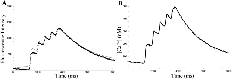
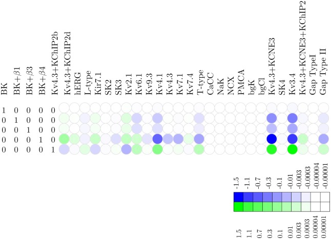
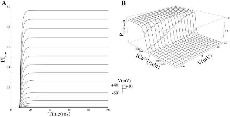
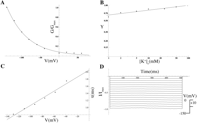
Uterine smooth muscle cells remain quiescent throughout most of gestation, only generating spontaneous action potentials immediately prior to, and during, labor. This study presents a method that combines transcriptomics with biophysical recordings to characterise the conductance repertoire of these cells, the 'conductance repertoire' being the total complement of ion channels and transporters expressed by an electrically active cell. Transcriptomic analysis provides a set of potential electrogenic entities, of which the conductance repertoire is a subset. Each entity within the conductance repertoire was modeled independently and its gating parameter values were fixed using the available biophysical data. The only remaining free parameters were the surface densities for each entity. We characterise the space of combinations of surface densities (density vectors) consistent with experimentally observed membrane potential and calcium waveforms. This yields insights on the functional redundancy of the system as well as its behavioral versatility. Our approach couples high-throughput transcriptomic data with physiological behaviors in health and disease, and provides a formal method to link genotype to phenotype in excitable systems. We accurately predict current densities and chart functional redundancy. For example, we find that to evoke the observed voltage waveform, the BK channel is functionally redundant whereas hERG is essential. Furthermore, our analysis suggests that activation of calcium-activated chloride conductances by intracellular calcium release is the key factor underlying spontaneous depolarisations.

Fig 1. Model diagram.

(A) Diagrammatic representation of all potential entities considered in the model repertoire according to mRNA expression data [13]. (B) Diagrammatic representation of the potential entities based on the most parsimonious solution (ℓ₁-norm; see text for further details). SR: sarcoplasmic reticulum; CaCC: calcium-activated chloride channel; CaT: T-type calcium channel; CaL: L-type calcium channel; hERG: human ether-à-go-go-related gene potassium channel; Kvx.x: potassium channel; SK-x: “small unitary current” potassium channels; BK-x: “big unitary current” potassium channels; NCX: sodium-calcium exchanger; PMCA: plasma-membrane calcium exchanger; pNaK: sodium-potassium exchanger; bgK: background potassium current; bgCl: background chloride current.

Fig 2. Calcium dynamics.

(A) Calcium fluorescence signal (dots) together with the least-squares fit of the calcium excitation model (solid line); parameter estimates are given in Table 4. (B) Reconstructed calcium concentration time course obtained using the model with these estimates.

Fig 3. Validation of the model.

(A) Bar chart comparing experimental and simulated Kv2.1, hERG, and Kir7.1 current densities (means±SEM). (B, C, D) ScTx-, dofetilide-, and VU590-sensitive currents in day-15 (D15) mice samples, the asterisk indicating at which point in time the current was sampled for the data reported in A; experimental traces under voltage-clamp conditions with 40 mV voltage step for ScTx- and dofetilide-sensitive currents and −150 mV for VU590-sensitive current from holding potential of −60 mV (ScTx: n = 19; dofetilide: n = 7; VU590: n = 9). A detailed comparison of measured and simulated currents is reported in S1 Fig. Voltage time series data are provided in S2 Data.

Fig 4. Redundancy map for the BK potassium channel.

Heat map of the null space matrix in echelon form with BK as a leading variable, showing which linear combinations of other channels can compensate for shifts in BK density. Whereas shifts in the BK_α density require virtually no compensation to maintain the voltage waveform, shifts in e.g. BK_α + β4 require large compensatory shifts in several other channels, both upward and downward. The color key relates hue to the log₁₀ of the fold change.

Fig 5. Redundancy map for the hERG potassium channel.

Heat map of the null space matrix in echelon form with hERG as a leading variable, showing which linear combinations of other channels can compensate for shifts in BK density. Shifts in e.g. hERG require large compensatory shifts in several other channels. The color key relates hue to the log₁₀ of the fold change.

Fig 6. The effect of a shift in the BK channel density on the action potential.

The effect of varying the BK channel density on the action potential triggered by a 10-sec extracellular ATP step function, compared to compensatory corrections of the densities of the various other channels according to the redundancy map shown in Fig 4. The solid line shows the reference waveform, which is produced by running the simulation model in free-running mode with parameter values constrained by the ℓ₁-norm. The dashed line shows the distortion caused by a small change in BK density, while the dotted line shows the waveform when compensatory shifts in other channels are applied in addition to the BK perturbation, partially restoring the waveform back to the reference waveform. (i) enlarged detail.

Fig 7. Effect of a shift in the SK₂ channel density on the action potential.

The effect of varying the SK₂ channel density on the action potential triggered by a 10-sec extracellular ATP step function, compared to compensatory corrections of the densities of the various other channels according to the redundancy map. The solid line shows the reference waveform, which is produced by running the simulation model in free-running mode with parameter values constrained by the ℓ₁-norm. The dashed line shows the distortion caused by a small change in SK₂ density, while the dotted line shows the waveform when compensatory shifts in other channels are applied in addition to the SK₂ perturbation, partially restoring the waveform back to the reference waveform. (i, ii) enlarged details.

Fig 8. Properties of I_P2X4.

(A) Normalised I_P2X4 theoretical current traces for various ATP concentrations at a holding potential of −60 mV. (B) Simulated ATP-concentration effect curve (solid line) and experimental data by Toulme et al [38] (solid circles). Values are normalised to the peak current values.

Fig 9. Effect of increasing the extracellular ATP concentration.

Simulation of the mathematical model in free-running mode, showing the effect of increasing the extracellular ATP concentration on the myometrium AP waveform. Key to ATP concentrations during 10-sec application: light blue: nil; blue: 10 μM; black: 100 μM; green: 1 mM; and red: 10 mM.

Fig 10. Effect of 5-BDBD on mechanical activity.

(A) Representative trace of force generated by human myometrium at term, registered before and during application of 5-BDBD. (B) Reduction of contraction frequency associated with application of 5-BDBD (n = 11, means±SEM, p < 0.001).

Fig 11. Effect of PIP₂ on the Kir7.1 G-V curve.

Simulated PIP₂ effect on G-V curve (solid line) with data extracted from experiments by Pattnaik et al [56] (solid circles). The G-V curve in the absence of PIP₂ (dashed line) is shown for comparison.

Fig 12. Simulations in support of Hypothesis III.

(A) Simulated local calcium sparks; the panel to the right is an expanded time-axis representation of the boxed section (i). (B) Train of action potentials in response to driving the gating kinetics of a small proportion (5%) of the CaCC population with the simulated calcium sparks on top of the global cytosolic calcium concentration.

Fig 13. Model simulations in free-running mode.

(A) Action potential triggered by a 10-sec extracellular ATP step function from 0 to 15 μM with parameter values constrained by the ℓ₁-norm. (B) Effect of setting the channel densities of BK and its isoforms to zero. (C) Effect of doubling the channel densities of BK and its isoforms. (D) Effect of setting the channel density of the Kv2.1 channel to zero. (E) Effect of doubling the channel density of Kv2.1.

Fig 14. ScTx modulates AP frequency, duration, and spike amplitude.

Spontaneous electrical activity recorded from the longitudinal layer of D15 & D18 murine myometrium (A, B). Activity consisted of slow depolarisation to threshold, followed by an action potential composed of a plateau upon which a number of spikes were superimposed. The bar represents the maximum effect in the presence of 100 nM ScTx. (C) Mean AP spike amplitude increase from 42.87±5.07 mV to 53.25±3.78 mV (p ≤ 0.05) in D15 tissue (n = 6) and from 45.5±4.96 mV to 56.21±3.37 mV in D18 tissue (n = 6). (D) Decrease in mean AP duration from 16.77±2.14 s to 11.87±0.76 s (p ≤ 0.05) in D15 tissue but no significant difference in D18 tissue. (E) Application of 100 nM of ScTx increased AP frequency in the D15 samples from a mean of 1.69±0.18 to 2.31±0.34 AP min⁻¹ and from 1.11±0.22 to 1.38±0.19 AP min⁻¹ in D18 tissue. (F) ScTx did not alter the resting membrane potential of either D15 or D18 (p ≤ 0.01).

Fig 15. Kv2.1 contribution to spontaneous contractile activity.

(A, B) Representative isometric force recordings in the presence of 100 nM ScTx in D15 (A) and D18 (B). (C) ScTx significantly increases contraction amplitude in both D15 murine myometrium from 13.32±1.79 mN to 14.24±1.87 mN and in D18 from 9.69±1.79 mN to 11.02 ± 1.87 mN. (D) ScTx significantly decreases contraction half width in D15 from 22.97±1.38s to 17.65±1.86s, while contraction half width in D18 tissue remained unchanged. (E) Effect of ScTx on contraction frequency for D15 & D18 murine myometrium. ScTx significantly increased contraction frequency for D15 & D18 murine myometrium from 0.74±0.05 to 0.89±0.07 contractions per minute and in D18 from 0.82±0.06 to 0.99±0.07 contractions per minute (p ≤0.01, n = 7).

Fig 16. Experimental I–V relationships.

Replicate I–V curves (n = 5 cells) measured under voltage-clamp conditions; values are averages over a 50 ms period, commencing 450 ms after applying a voltage step.

Fig 17. Properties of I_Kv2.1.

(A) Normalised I_Kv2.1 current trace in simulated voltage-clamp experiments. Currents are recorded during 1 s voltage steps to potentials ranging from −50 to +80 mV from a holding potential of −60 mV. (B) Data from Frech et al [79] peak I–V curve (solid squares) obtained from the series of experiments shown in (A); compared to simulation (solid triangles). Values are normalised to the peak current value.

Fig 18. State transition diagram of the Markov model for the Kv2.1 channel.

$C_0^{\text{[Kv2.1]}}$–$C_4^{\text{[Kv2.1]}}$ are the closed states; O^[Kv2.1] is the open state, and $I_0^{\text{[Kv2.1]}}$–$I_5^{\text{[Kv2.1]}}$ are the inactivation states; $k_v^{\text{[Kv2.1]}}$, $k_{-v}^{\text{[Kv2.1]}}$, $k_1^{\text{[Kv2.1]}}$, $k_{-1}^{\text{[Kv2.1]}}$, $k_0^{\text{[Kv2.1]}}$, and $k_{-0}^{\text{[Kv2.1]}}$ denote transition rates between the states.

Fig 19. Properties of I_Kv9.3.

(A) Normalised I_Kv9.3 current trace in simulated voltage-clamp experiments. Currents are recorded during 1 s voltage steps to potentials ranging from −50 to 80 mV from a holding potential of −60 mV. (B) Simulated (solid triangles) peak I–V relationship obtained from the series of experiments shown in (A). Values are normalised to the peak current value. (C) Steady state activation and inactivation curves from Patel et al [15]. (D) Simulated activation time constant derived from experimental data (filled circles) from Patel et al [15].

Fig 20. Properties of I_Kv6.1.

(A) Normalised I_Kv6.1 current trace in simulated voltage-clamp experiments. Currents are recorded during 1 s voltage steps to potentials ranging from −50 to 80 mV from a holding potential of −60 mV. (B) Simulated (solid triangles) peak I–V relationship obtained from the series of experiments shown in (A). Values are normalised to the peak current value. (C) Steady state activation and inactivation curves from Kramer et al [16]. (D) Simulated activation time constant derived from experimental data (filled circles) from Patel et al [15].

Fig 21. Properties of I_Kv3.4.

(A) Normalised I_Kv3.4 current trace in simulated voltage-clamp experiments. Currents are recorded during 1 s voltage steps to potentials ranging from −50 to 80 mV from a holding potential of −60 mV. (B) Steady state activation and inactivation curves from Rudy et al [28] (C) Simulated time-to-peak derived from data (filled circles) from Rudy et al [28]. (D) Simulated inactivation time constant derived from experimental data (filled circles) from Rudy et al [28].

Fig 22. Properties of I_Kv4.1.

(A) Normalised I_Kv4.1 current trace in simulated voltage-clamp experiments. Currents are recorded during 1 s voltage steps to potentials ranging from −50 to 80 mV from a holding potential of −60 mV. (B) Steady state activation and inactivation curves from Jerng et al [29]. (C) Simulated time-to-peak derived from data (filled circles) from Nakamura et al [30]. (D) Simulated inactivation time constants derived from experimental data (filled circles) from Jerng et al [29].

Fig 23. State transition diagram of the Markov model for the Kv4.3 channel.

$C_0^{\text{[Kv4.3]}}$–$C_4^{\text{[Kv4.3]}}$ are the closed states; O^[Kv4.3] is the open state and $I_0^{\text{[Kv4.3]}}$–$I_6^{\text{[Kv4.3]}}$ are the inactivation states; α^[Kv4.3], β^[Kv4.3], $k_{ci}^{\text{[Kv4.3]}}$, $k_{ic}^{\text{[Kv4.3]}}$, $k_{oc}^{\text{[Kv4.3]}}$, $k_{co}^{\text{[Kv4.3]}}$, $k_{56}^{\text{[Kv4.3]}}$ and $k_{65}^{\text{[Kv4.3]}}$ denote transition rates between the states.

Fig 24. Properties of I_Kv4.3.

(A) Normalised I_Kv4.3 current trace in simulated voltage-clamp experiments. Currents are recorded during 1 s voltage steps to potentials ranging from −50 to 80 mV from a holding potential of −60 mV. (B) Simulated (solid triangles) peak I–V relationship obtained from the series of experiments shown in (A). Values are normalised to the peak current value.

Fig 25. State transition diagram of the Markov model for the hERG channel.

$C_1^{\text{[hERG]}}$–$C_3^{\text{[hERG]}}$ are closed states, O^[hERG] is the open state and I^[hERG] the inactivation state.

Fig 26. Properties of I_hERG.

(A) Simulated I_hERG current trace in simulated voltage-clamp experiments. Currents are recorded during 1 s voltage steps to potentials ranging from −50 to 80 mV from a holding potential of −60 mV. Values are normalised to the peak current value. (B) Simulated I–V relationship obtained from the series of experiments shown in (A) at t = 400 ms. Values are normalised to the peak current value at the same time point. (C) Simulated peak tail I–V relationship obtained from the series of experiments shown in (A). Values are normalised to the peak tail current value.

Fig 27. State transition diagram of the Markov model for the effect of PIP₂ on the hERG channel.

$C_1^{\text{[hERG]}}$–$C_3^{\text{[hERG]}}$ are closed states, O^[hERG] is the open state, and I^[hERG] the inactivation state. The transition rates have different values depending on whether PIP₂ is absent or present [55].

Fig 28. Properties of I_Kv7.1.

(A) Simulated voltage clamp traces of homomeric Kv7.1 channel from holding potential of −60 mV, where the voltage was stepped to values up to +80 mV in 10 mV increments. (B) Simulated peak I–V relationship obtained from the voltage clamp experiments shown in (A). Values are normalised to the peak current values.

Fig 29. State transition diagram of the Markov model for the Kv7.1 channel.

$C_1^{\text{[Kv7.1]}}$–$C_2^{\text{[Kv7.1]}}$ are the closed states, $O_1^{\text{[Kv7.1]}}$–$O_2^{\text{[Kv7.1]}}$ are the open states and I^[Kv7.1] the inactivation state. ${\alpha }_1^{\text{[Kv7.1]}}$, ${\beta }_1^{\text{[Kv7.1]}}$, ${\alpha }_2^{\text{[Kv7.1]}}$, ${\beta }_2^{\text{[Kv7.1]}}$, λ^[Kv7.1], μ^[Kv7.1], δ^[Kv7.1], and ϵ^[Kv7.1] denote transition rates between the states.

Fig 30. Properties of I_Kv7.4.

(A) Simulated voltage clamp traces of homomeric Kv7.4 channel at 28°C from holding potential of −90 mV, where the voltage was stepped to values up to +40 mV in increments of 10 mV, subsequently stepped down to −120 mV. (B) Steady state activation curves from Miceli et al [96]. (C) Simulated activation fast time constant derived from experimental data (filled circles) from Schröder et al [34].

Fig 31. State transition diagram of the Markov model for the BK_α channel.

State transition diagram of the Markov model for the BK_α channel. $C_1^{\text{[BK]}}$–$C_4^{\text{[BK]}}$ are the closed states and $O_1^{\text{[BK]}}$–$O_4^{\text{[BK]}}$ are the open states. Horizontal transitions represent voltage sensor movement while vertical transitions represent channel opening.

Fig 32. Properties of I_BKα.

(A) Simulated voltage clamp traces of α-subunit BK channel from holding potential of −80 mV, where the voltage was stepped to values up to +240 mV in 10 mV increments. (B) Simulated open-channel probability plotted against [Ca²⁺]_i and the membrane potential.

Fig 33. Properties of I_BKα+β1.

(A) Simulated voltage clamp traces of BK_α+β1 channel from holding potential of −80 mV, where the voltage was stepped to values up to +240 mV in increments of 10 mV, in the absence of calcium. (B) Simulated open-channel probability plotted against [Ca²⁺]_i and the membrane potential.

Fig 34. Properties of I_BKα+β3.

(A) Simulated voltage clamp traces of BK_α+β3 channel from holding potential of −180 mV, where the voltage was stepped to values up to +80 mV in 10 mV increments for various μM [Ca²⁺]_i, then stepped back to −180 mV (B) Simulated steady-state I−V relationship obtained from the series of voltage clamp experiments shown in (A). Values are normalised to the peak current values.

Fig 35. State transition diagram of the Markov model for the BK_α+β3 channel.

$C_n^{[\alpha +\beta 3]}$ is the closed state, $O_n^{[\alpha +\beta 3]}$ is the open state, and $I_n^{[\alpha +\beta 3]}$ is the inactivation state (n = 1…5); k_f, k_r, k_b, and k_u denote transition rates between the states.

Fig 36. Properties of I_BKα+β4.

(A) Simulated voltage clamp traces of BK_α+β4 channel from holding potential of −80 mV, where the voltage was stepped to values up to +80 mV in 10 mV increments in 10 μM [Ca²⁺]_i (B) Simulated peak I–V relationship obtained from the series of voltage clamp experiments shown in (A). Values are normalised to the peak current values.

Fig 37. Properties of I_SK2.

(A) Activation variable as a function of [Ca²⁺]_i obtained from experimental data of Hirschberg et al [22] as function of [Ca²⁺]_i. (B) Activation time constant obtained from simulated current traces as function of [Ca²⁺]_i.

Fig 38. Properties of I_SK3.

(A) Simulated voltage clamp traces of SK3 channel from holding potential of −80 mV, where the voltage was stepped to test potential up to +80 mV in 10 mV increments in 5 μM [Ca²⁺]_i (B) Activation variable obtained from experimental data of Xia et al [23] as function of [Ca²⁺]_i.

Fig 39. Properties of I_Kir7.1.

(A) Steady state activation curve from Doring et al [35] fit by a single exponential. (B) Double logarithmic plot for the Kir7.1 conductance as a function of [K⁺]_o. (C) Activation time constant derived from experimental data (filled circles) from Doring et al [35]. (D) Current trace in simulated voltage-clamp experiments. Currents are recorded during 1 s voltage steps to potentials up to −150 mV from a holding potential of 0 mV. Values are normalised to the peak current values.

Fig 40. Properties of I_L-type.

(A) Normalised I_L-type current trace in simulated voltage-clamp experiments. Currents are recorded during 1 s voltage steps to potentials ranging from −50 to 80 mV from a holding potential of −50 mV. (B) Simulated (solid triangles) peak I–V relationship obtained from the series of experiments shown in (A). Values are normalised to the peak current values, data (circles) from Blanks et al [112]. (C) Steady state activation and inactivation curves. (D) Simulated activation and inactivation time constant.

Fig 41. Properties of I_T-type.

(A) Normalised I_T-type current trace in simulated voltage-clamp experiments. Currents are recorded during 1 s voltage steps to potentials ranging from −60 to 80 mV from a holding potential of −60 mV. (B) Simulated (circles) peak I–V relationship obtained from the series of experiments shown in (A). Values are normalised to the peak current values. (C) Steady state activation and inactivation curves. (D) Simulated activation and inactivation time constant.

Fig 42. Properties of I_CaCC.

(A) Normalised I_CaCC current trace in simulated voltage-clamp experiments. Currents are recorded during 1 s voltage steps to potentials ranging from −120 to 140 mV from a holding potential of 0 mV then followed by a repolarising pulse to −140 mV. (B) Simulated steady-state I–V relationship obtained from the series of experiments shown in (A). Values are normalised to the peak current values. (C) [Ca²⁺]_i-dependence of CaCC channel activation. Conductance as a function of [Ca²⁺]_i at −66 mV and +74 mV, respectively.

Fig 43. Properties of the gap junctions in MSMC.

Simulated currents for Type I and Type II are shown in (A) and (B), respectively. The currents are elicited in response to 5 s square pulses in the voltage range of ± 90 mV from holding potential of 0 mV. Steady-state conductance as function of V_j for Type I an Type II shown in (C) and (D), respectively, using quasi-symmetrical Boltzmann functions (dashed line) and the Gaussian function (solid line). The time constant as function of V_j for Type I and Type II are shown in (E) and (F), respectively.

References

1. Hille B (2001) Ion Channels of Excitable Membranes, Third Edition Sinauer Associates, Inc.
1. ten Tusscher K, Noble D, Noble PJ, Panfilov AV (2004) A model for human ventricular tissue. Am J Physiol Heart Circ Physiol 286: H1573–H1589. - PubMed
1. Livshitz L, Rudy Y (2009) Uniqueness and stability of action potential models during rest, pacing, and conduction using problem-solving environment. Biophys J 97: 1265–1276. 10.1016/j.bpj.2009.05.062 - DOI - PMC - PubMed
1. Tong WC, Choi CY, Karche S, Holden AV, Zhang H, et al. (2011) A computational model of the ionic currents, Ca2+ dynamics and action potentials underlying contraction of isolated uterine smooth muscle. PLoS ONE 6(4): e18685 10.1371/journal.pone.0018685 - DOI - PMC - PubMed
1. Andersen H, Barclay M (1995) A computer model of uterine contractions based on discrete contractile elements. Obstet Gynecol 86: 108–111. 10.1016/0029-7844(95)00111-4 - DOI - PubMed
Publication types