

Assessing the robustness of spatial pattern sequences in a dryland vegetation model
- PMID: 27118924
- PMCID: PMC4841491
- DOI: 10.1098/rspa.2015.0893
Assessing the robustness of spatial pattern sequences in a dryland vegetation model
Abstract
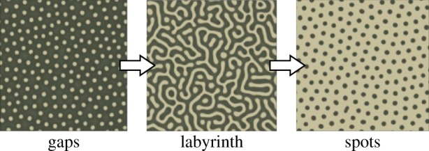
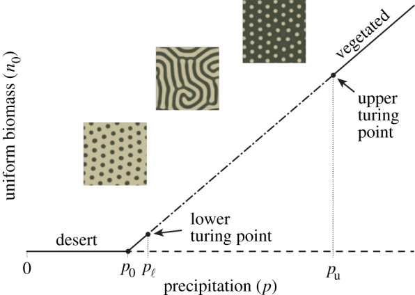
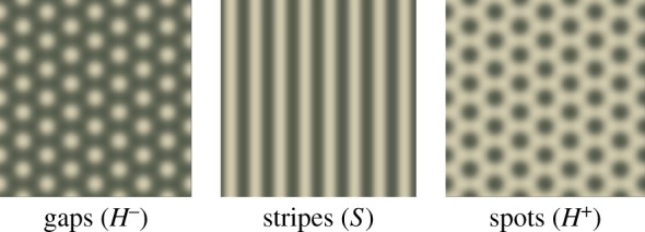
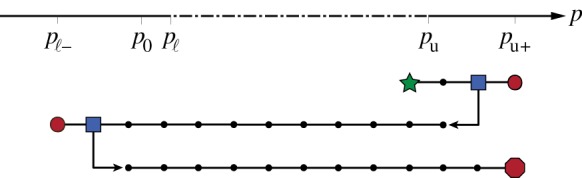
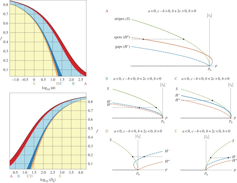
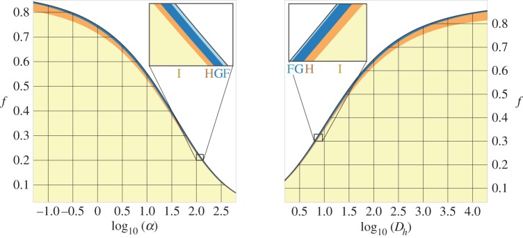
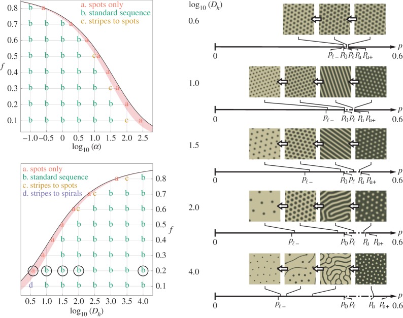
A particular sequence of patterns, 'gaps→labyrinth→spots', occurs with decreasing precipitation in previously reported numerical simulations of partial differential equation dryland vegetation models. These observations have led to the suggestion that this sequence of patterns can serve as an early indicator of desertification in some ecosystems. Because parameter values in the vegetation models can take on a range of plausible values, it is important to investigate whether the pattern sequence prediction is robust to variation. For a particular model, we find that a quantity calculated via bifurcation-theoretic analysis appears to serve as a proxy for the pattern sequences that occur in numerical simulations across a range of parameter values. We find in further analysis that the quantity takes on values consistent with the standard sequence in an ecologically relevant limit of the model parameter values. This suggests that the standard sequence is a robust prediction of the model, and we conclude by proposing a methodology for assessing the robustness of the standard sequence in other models and formulations.
Keywords: desertification; dryland ecosystems; early-warning signs; models of vegetation pattern formation; pattern formation.
Figures
Similar articles
-
Desertification by front propagation?J Theor Biol. 2017 Apr 7;418:27-35. doi: 10.1016/j.jtbi.2017.01.029. Epub 2017 Jan 20. J Theor Biol. 2017. PMID: 28115204
-
Transitions between patterned states in vegetation models for semiarid ecosystems.Phys Rev E Stat Nonlin Soft Matter Phys. 2014 Feb;89(2):022701. doi: 10.1103/PhysRevE.89.022701. Epub 2014 Feb 3. Phys Rev E Stat Nonlin Soft Matter Phys. 2014. PMID: 25353503
-
A topographic mechanism for arcing of dryland vegetation bands.J R Soc Interface. 2018 Oct 10;15(147):20180508. doi: 10.1098/rsif.2018.0508. J R Soc Interface. 2018. PMID: 30305423 Free PMC article.
-
The role of refuges in the persistence of Australian dryland mammals.Biol Rev Camb Philos Soc. 2017 May;92(2):647-664. doi: 10.1111/brv.12247. Epub 2015 Dec 21. Biol Rev Camb Philos Soc. 2017. PMID: 26685752 Review.
-
A multi-scale perspective of water pulses in dryland ecosystems: climatology and ecohydrology of the western USA.Oecologia. 2004 Oct;141(2):269-81. doi: 10.1007/s00442-004-1570-y. Epub 2004 May 8. Oecologia. 2004. PMID: 15138879 Review.
Cited by
-
An integrodifference model for vegetation patterns in semi-arid environments with seasonality.J Math Biol. 2020 Sep;81(3):875-904. doi: 10.1007/s00285-020-01530-w. Epub 2020 Sep 4. J Math Biol. 2020. PMID: 32888058 Free PMC article.
-
Population mobility induced phase separation in SIS epidemic and social dynamics.Sci Rep. 2020 May 6;10(1):7646. doi: 10.1038/s41598-020-64183-1. Sci Rep. 2020. PMID: 32376877 Free PMC article.
-
Bounded risk disposition explains Turing patterns and tipping points during spatial contagions.R Soc Open Sci. 2024 Oct 2;11(10):240457. doi: 10.1098/rsos.240457. eCollection 2024 Oct. R Soc Open Sci. 2024. PMID: 39359464 Free PMC article.
-
Stabilizing a homoclinic stripe.Philos Trans A Math Phys Eng Sci. 2018 Nov 12;376(2135):20180110. doi: 10.1098/rsta.2018.0110. Philos Trans A Math Phys Eng Sci. 2018. PMID: 30420550 Free PMC article.
-
Pattern blending enriches the diversity of animal colorations.Sci Adv. 2020 Dec 2;6(49):eabb9107. doi: 10.1126/sciadv.abb9107. Print 2020 Dec. Sci Adv. 2020. PMID: 33268371 Free PMC article.
References
-
- von Hardenberg J, Meron E, Shachak M, Zarmi Y. 2001. Diversity of vegetation patterns and desertification. Phys. Rev. Lett. 87, 198101 (doi:10.1103/PhysRevLett.87.198101) - DOI - PubMed
-
- Bel G, Hagberg A, Meron E. 2012. Gradual regime shifts in spatially extended ecosystems. Theor. Ecol. 5, 591–604. (doi:10.1007/s12080-011-0149-6) - DOI
-
- Dakos V, Kéfi S, Rietkerk M, van Nes EH, Scheffer M. 2011. Slowing down in spatially patterned ecosystems at the brink of collapse. Am. Nat. 177, E153–E166. (doi:10.1086/659945) - DOI - PubMed
-
- Gilad E, von Hardenberg J, Provenzale A, Shachak M, Meron E. 2004. Ecosystem engineers: from pattern formation to habitat creation. Phys. Rev. Lett. 93, 098105 (doi:10.1103/PhysRevLett.93.098105) - DOI - PubMed
-
- Gowda K, Riecke H, Silber M. 2014. Transitions between patterned states in vegetation models for semi-arid ecosystems. Phys. Rev. E. 89, 022701 (doi:10.1103/PhysRevE.89.022701) - DOI - PubMed
LinkOut - more resources
Full Text Sources
Other Literature Sources
