Topology of ON and OFF inputs in visual cortex enables an invariant columnar architecture

Abstract

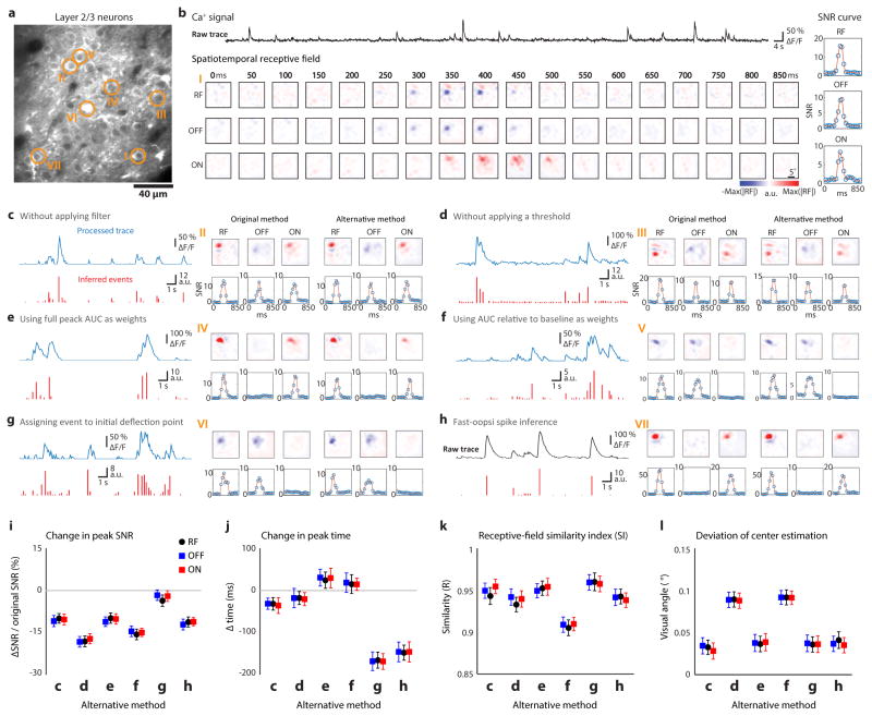
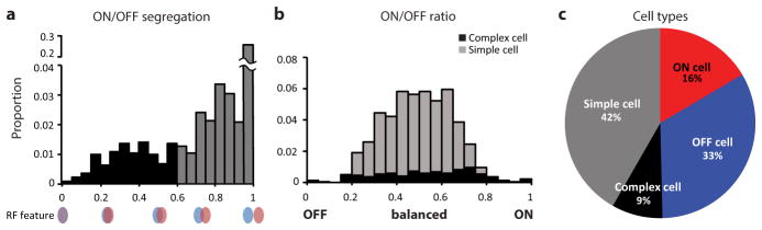
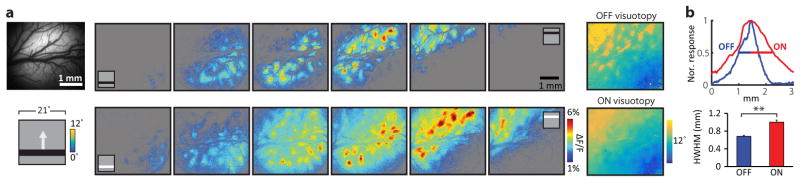
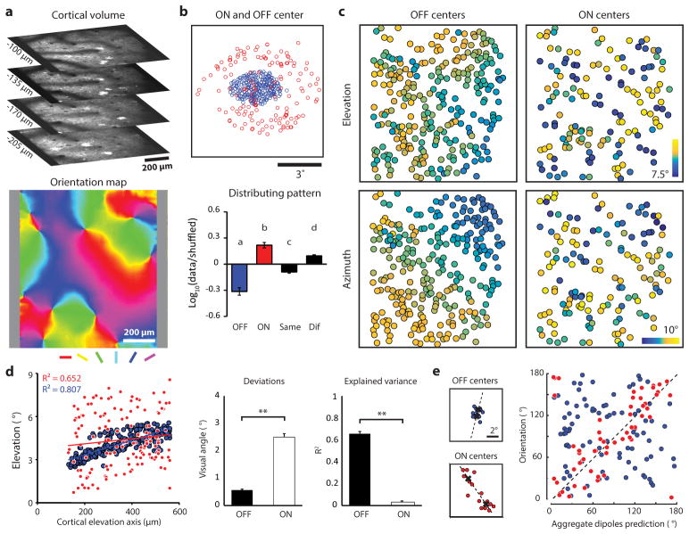
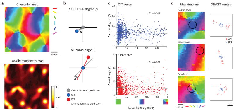
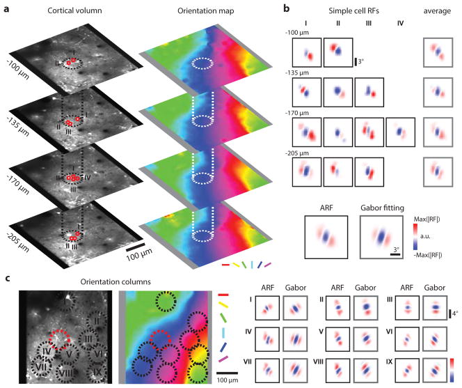
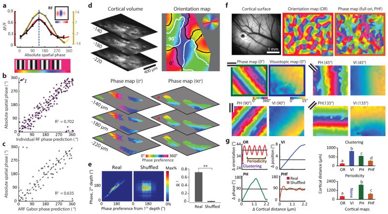
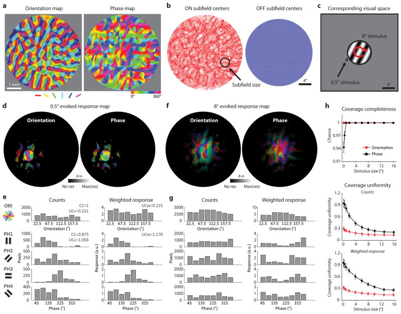
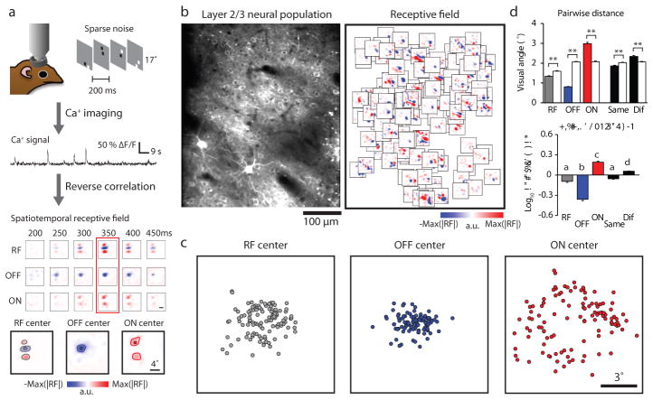
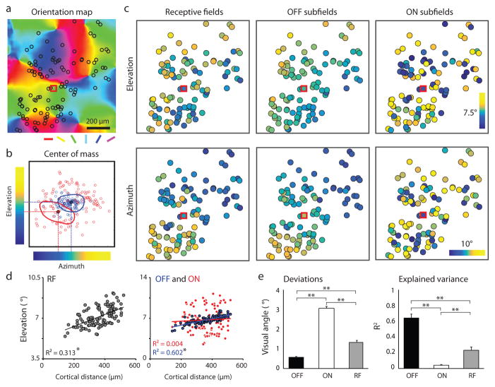
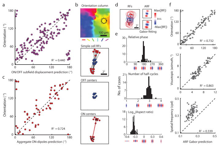
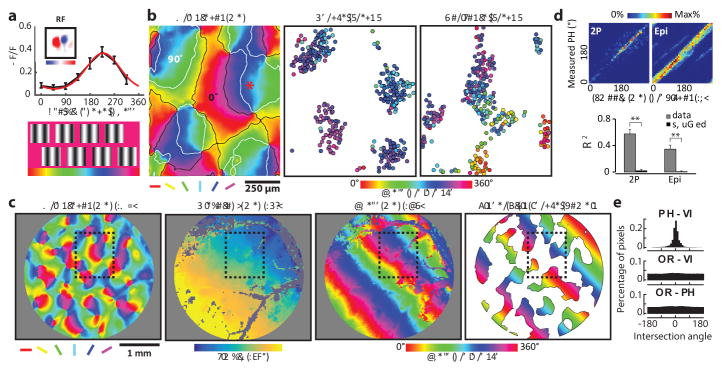
Circuits in the visual cortex integrate the information derived from separate ON (light-responsive) and OFF (dark-responsive) pathways to construct orderly columnar representations of stimulus orientation and visual space. How this transformation is achieved to meet the specific topographic constraints of each representation remains unclear. Here we report several novel features of ON-OFF convergence visualized by mapping the receptive fields of layer 2/3 neurons in the tree shrew (Tupaia belangeri) visual cortex using two-photon imaging of GCaMP6 calcium signals. We show that the spatially separate ON and OFF subfields of simple cells in layer 2/3 exhibit topologically distinct relationships with the maps of visual space and orientation preference. The centres of OFF subfields for neurons in a given region of cortex are confined to a compact region of visual space and display a smooth visuotopic progression. By contrast, the centres of the ON subfields are distributed over a wider region of visual space, display substantial visuotopic scatter, and have an orientation-specific displacement consistent with orientation preference map structure. As a result, cortical columns exhibit an invariant aggregate receptive field structure: an OFF-dominated central region flanked by ON-dominated subfields. This distinct arrangement of ON and OFF inputs enables continuity in the mapping of both orientation and visual space and the generation of a columnar map of absolute spatial phase.

Extended Data Figure 1. Robust receptive field estimation from GCaMP6 calcium signal in layer 2/3 neurons

a, Somatic location of seven example cells (circle) overlaid on the two-photon field of view. b, Raw calcium trace, spatiotemporal receptive field and signal-noise ratio (SNR) curve from an example cell in a. c–h, Six different ways to infer the onset time and response strength of neural activity were used to compare with the original method described in Methods for six example cells in a. Processed calcium trace before starting inference (blue) and the inferred response (red) are shown on the left. Receptive fields/SNR curves derived from original or alternative method are shown on the right. i–l, Change in peak SNR (i) and peak time (j), receptive field similarity index (k), deviation of the RF/subfields center estimation (l) illustrating that the main conclusions regarding receptive field structure and fine visuotopic organization are not altered by the signal processing method employed (N = 143 cells from 3 animals). All error bars indicate s.e.m.

Extended Data Figure 2. Cell type categorization in tree shrew primary visual cortex layer 2/3

a, Distribution of ON/OFF segregation index values for simple and complex cells (see Methods). A value of 0.6 was used to delineate the two classes. b, Distribution of ON/OFF ratio values for simple and complex cells. In both a and b, the proportions are based on the total number of cells; however, the single sign cell population is not shown in the plots. c, Percentage of different classes of neurons in tree shrew visual cortex layer 2/3.

Extended Data Figure 3. Cortical spread of light and dark evoked activity in epi-fluorescence imaging

a, The wide field epi-fluorescence imaging of visual cortex reveals a similar visuotopic progression for the zones of activity found for static light and dark bar stimuli at different locations in elevation. b, The bandwidth of the normalized cortical activity pattern, characterized by half width at half maximum (HWHM), shows that the light stimuli evoke broader cortical activity patterns than dark stimuli at the same visuotopic location (N = 21 stimulus-evoked response maps from 4 animals, P = 9.6 × 10^–5, rank-sum test). Error bars indicate s.e.m.

Extended Data Figure 4. ON and OFF receptive field organization of single sign cells

a, The cortical volume and the orientation map of an example imaging area. b, The ON and OFF centers from single sign cells display an arrangement similar to the simple cell population. The bottom plot shows that the distribution pattern of ON and OFF receptive fields is consistent with the ON- and OFF- subfields of the simple cell population (N = 8 imaging areas from 7 animals, Kruskal-Wallis test; compare with Fig 1c and d, letters indicating groups with statistically significant difference, P < 0.01). c, The visuotopic organization of ON and OFF receptive field centers was similar to the simple cell ON- and OFF- subfields. d, The relation between cortical distance and visuotopic position demonstrating the difference in visuotopic precision for ON and OFF receptive fields (linear regression). Deviations of the experimental results from the linear fit and explained variance of the smooth visuotopy (N = 16 visuotopic maps, combining elevation and azimuth results from 8 imaging areas, **p < 0.0001, rank-sum test) are consistent with the results from simple cell ON- and OFF subfields. e, Only the displacement of the population ON receptive field center, but not OFF receptive field center, can predict the orientation tuning of the orientation column (circular correlation, N = 68 cortical columns, P = 9.51 × 10^–3 for ON; N = 89 cortical columns, P = 0.586 for OFF). All error bars indicate s.e.m.

Extended Data Figure 5. Visuotopic arrangement of ON and OFF subfields is independent of orientation map structure

a, An example orientation map and local heterogeneity index map. The local heterogeneity index was used to compare ON and OFF subfield arrangement for cortical regions with different orientation map structure. b, (top) Illustration comparing the visuotopic displacement of OFF subfields to the theoretical prediction from a smooth visuotopic map. (bottom) Illustration comparing the visuotopic displacement of ON subfields to the orientation map. c, (top) Visuotopic distortion of OFF subfield centers in relation to the structure of the orientation map. There is no relationship between local heterogeneity and the visuotopic precision of OFF subfields (linear regression, N = 1811 cells from 7 animals, P = 8.2 × 10⁻²). (bottom) Axial mismatch of ON subfield centers in relation to the structure of the orientation map. There is no relationship between local heterogeneity and the axial displacement of ON subfield centers (linear regression, N = 1811 cells, P = 9.6 × 10⁻²). d, Examples of the ON and OFF subfield center distributions from an 80 μm circular region (black circle) centered on three distinct regions of orientation map.

Extended Data Figure 6. Contribution of simple cells at different depths to aggregate receptive field of cortical column

a, An example orientation column at four depths, with two-photon images on the left and the corresponding orientation maps on the right. b, Simple cell receptive fields from these four cortical depths. Each RF was normalized by the strongest subfield. The average of the RFs within each depth appear similar. All the RFs within the orientation column were then pooled into an aggregate receptive field (ARF) and then fitted with 2D Gabor function. c, Other nine examples of ARFs from different orientation columns display the same organization: OFF subfield in the center with ON subfields flanking on two sides.

Extended Data Figure 7. Characterizing spatial phase tuning, phase column, and phase map

a, The phase tuning from an example cell (black) and its Gaussian fit (red) compared with the phase tuning curve predicted from its receptive field structure (gray) and its Gaussian fit (yellow). Dashed line depicts the preferred phase derived from the Gaussian fit to the experimental data. b, Relation of absolute phase prediction from receptive field structure to absolute phase tuning measurement (N = 179 cells from 2 animals, P = 1.8 × 10^–18, circular regression). c, Phase preference of the orientation column is well predicted by the phase parameter of the Gabor fit to the ARF (N = 73 cortical columns from 5 animals, P = 1.7 × 10^–10, circular regression). d, Example two-photon phase maps derived from pixel tuning at three cortical depths for both horizontal and vertical orientations. e, Comparison of phase preference from different cortical depths (red asterisks in d) showing the consistence of columnar structure for spatial phase (rank-sum test for R² from circular regression, N = 36 pairs of maps at different depths from 2 animals, P = 8.2 × 10^–18). f, Large scale functional maps visualized by epi-fluorescence imaging. The phase map with full orientation coverage (right) was constructed from four individual phase maps measured independently with four orientations (0°, 45°, 90°, 135°). The phase maps for single orientations with corresponding visuotopic maps are shown separately in lower two rows. g, The statistical structure of functional maps (orientation, phase, visuotopy, and phase with 4 orientations) summarized by the relationship between the change in cortical distance and the average change in preferred feature (left). Summary comparison of clustering and periodicity of the preferred features of four functional maps from 6 animals (right). Each map exhibits distinct clustering and periodicity (N = 32 sample regions from 6 animals, Kruskal-Wallis test with post hoc using Dunn’s method, letters indicating groups with statistically significant difference, P < 0.05). All error bars indicate s.e.m.

Extended Data Figure 8. Simulation based on experimental observations to evaluate completeness and uniformity of coverage for orientation and phase representations

a, The large scale orientation preference map derived from intrinsic signal imaging and corresponding phase map predicted from experimental observations (see Methods). b, Distribution of ON and OFF subfield centers in visual space predicted from the visuotopic precision and orientation specific displacement demonstrated in this study. Although the distribution of the ON subfield centers in visual space appears uneven, complete coverage of visual space is achieved when the actual size of the ON subfields is considered. c, Illustration of two of the visual stimuli (8 degree stimulus in the center, 0.5 degree stimulus to the left) used to simulate the evoked response map. d, Theoretical stimulus evoked orientation and phase response maps for sample 0.5° stimulus shown in c (see Methods). e, Histograms showing the distribution of preferred orientation and phase values for pixels activated in d, calculated by counts of the pixels in the responsive region (left) or weighted by the strength of the responses (right). f, Theoretical stimulus evoked orientation and phase response maps for sample 8° stimulus shown in c (see Methods). g, Histograms showing the distribution of preferred orientation and phase values for pixels activated in f, calculated by counts of the pixels in the responsive region (left) or weighted by the strength of the responses (right). h, Completeness (top) and uniformity (middle, bottom) of coverage simulated with visual stimuli of various sizes and positions. Complete coverage can be achieved with stimuli of 1 degree, while coverage uniformity continues to improve with increases in stimulus size. The results of spatial phase were always the average results obtained with four different orientations. Error bars indicate s.e.m.

Figure 1. Differential arrangement of simple cell ON and OFF subfields in visual space

a, Spatiotemporal receptive fields and ON/OFF subfields of cortical neurons were independently obtained using calcium imaging combined with reverse correlation to a sparse noise stimulus. The receptive field and ON/OFF subfields were defined at the peak SNR time window. Small circles indicate the centers of mass of the whole RF and the ON/OFF subfields (see Methods). b, An example of a two-photon field of view and all the significant receptive fields (same scale as receptive fields in a) from individual cells overlaid on their soma locations. c, An example of the distribution of RF and OFF/ON subfield centers in visual space. d, The pairwise distance between the centers of mass for all categories and for shuffled data (white bars) from the example in c. Receptive fields, OFF subfields, and subfields sharing the same signs are more clustered while ON subfields and subfields with different signs are more scattered than by chance (rank-sum test for each group, **p < 0.0001). The bottom plot summarizes the comparison of real and shuffled data where positive values indicate a scattered distribution pattern and negative values indicate clustered distribution pattern relative to random shuffles (N = 8 fields of view from 7 animals, P = 6.1 5 10^–21, Kruskal-Wallis test with post hoc using Dunn’s method; letters indicating groups with statistically significant difference, P < 0.01, see Methods). Error bars indicate s.e.m.

Figure 2. Differences in visuotopic precision of simple cell ON and OFF subfield centers

a, Example field of view showing somatic location of all simple cells from four cortical depths (black circles) superimposed on the orientation map. b, The location in visual space of the center of mass of ON and OFF subfields for neurons in a illustrating the color code that is used to depict azimuth and elevation values in c. RF of an example cell (red square in a and c) showing translation of ON and OFF subfield centers into elevation-azimuth coordinates. c, The visual field location (elevation and azimuth) for the receptive field and ON/OFF subfields for each neuron illustrated in a. d, The relation between cortical distance (along the elevation axis) and elevation in visual space for the receptive fields (left) and the ON and OFF subfields (right) from the example in c. (linear regression, *P < 0.0001). e, The summary showing the deviations of the experimental data from smooth visuotopy (left) and the degree to which a smooth visuotopy accounts for the variance in the experimental data (right) (Kruskal-Wallis test with post hoc using Dunn’s method, N = 16 visuotopic maps, combining elevation and azimuth results from 8 imaging areas, **P < 0.0001; see Methods). Error bars indicate s.e.m.

Figure 3. Orientation columns exhibit an invariant aggregate receptive field structure

a, Consistent with simple cells in other mammals, the ON/OFF subfield displacement in visual space predicts the preferred orientation in individual cells (linear regression, N = 176 cells from 2 animals, P < 0.0001). b, Example of receptive fields from the simple cells in a single orientation column (dashed circle). Lines connect the ON subfield (red) and the OFF subfield (blue) centers of individual simple cell receptive fields. The ON centers form two clusters that define the aggregate ON-dipole of the column. c, The aggregate ON- dipoles from all the simple cells within individual orientation columns predicts the preferred orientation of the column (linear regression, P < 0.0001). d, The normalized simple cell receptive fields from a single column in b were averaged to derive the aggregate receptive field (ARF) which was fit with a Gabor. e, Cortical columns exhibit an invariant ARF structure resembling an OFF centered simple cell receptive field with specific relative phase, number of half-cycles, and aspect ratio. f, The parameters of the ARF Gabor fit account for multiple features of the cortical column including orientation, visual position, and spatial frequency (N = 73 cortical columns from 5 animals, circular or linear regression, all P < 0.0001; see Methods).

Figure 4. Smooth progression of absolute spatial phase across orientation domains

a, The phase tuning curve (black) and its Gaussian fit (red) for an example neuron derived from 8 static grating stimuli. b, Organization of the phase preference for populations of neurons derived with vertical and horizontal grating stimuli visualized with two-photon imaging at three cortical depths. Cortical domains with a significant response to vertical and horizontal gratings are delineated by contours (white and black respectively). Neighboring neurons exhibit similar phase preferences, and the preferences shift in a progressive fashion across the orientation domains. c, Epi-fluorescence imaging demonstrates relation of phase map derived with vertical grating to maps of orientation and visual space (azimuth). Black rectangle indicates the 2-P field of view shown in b. The smooth progression of preferred phase along the visuotopic axis orthogonal to the stimulus orientation is evident at this scale. The rightmost figure shows a linear fit of the phase signal within vertical orientation domains to approximate the phase preference map. d, Both for the two-photon and epi-fluorescence data, a smooth phase progression generated with a linear fit was used to test for correlation with the experimental data (circular regression, both P < 0.0001). The smooth progression accounted for a greater amount of the variance in the experimental data compared to shuffled data (**p < 0.0001, rank-sum test within group; see Methods). Error bars indicate s.e.m. e, The intersection of the phase and visuotopic map gradients shown in c peaks around 0 degree (0.32° in this case and −0.08° on average of six maps), indicating a parallel relationship (P = 5.2 × 10^–16, Rayleigh test), while there is no significant non-uniformity for the intersection of orientation map gradients with either phase or visuotopic map gradients (P > 0.05, Rayleigh test).

References

1. Hubel DH, Wiesel TN. Receptive fields, binocular interaction and functional architecture in the cat’s visual cortex. J Physiol (Lond) 1962;160:106–154. - PMC - PubMed
1. Ferster D, Chung S, Wheat H. Orientation selectivity of thalamic input to simple cells of cat visual cortex. Nature. 1996;380:249–252. - PubMed
1. Jin JZ, et al. On and off domains of geniculate afferents in cat primary visual cortex. Nat Neurosci. 2008;11:88–94. - PMC - PubMed
1. Jin J, Wang Y, Swadlow HA, Alonso JM. Population receptive fields of ON and OFF thalamic inputs to an orientation column in visual cortex. Nat Neurosci. 2011;14:232–238. - PubMed
1. Bosking WH, Crowley JC, Fitzpatrick D. Spatial coding of position and orientation in primary visual cortex. Nat Neurosci. 2002;5:874–882. - PubMed
Publication types