Epidemic spreading with activity-driven awareness diffusion on multiplex network

Abstract

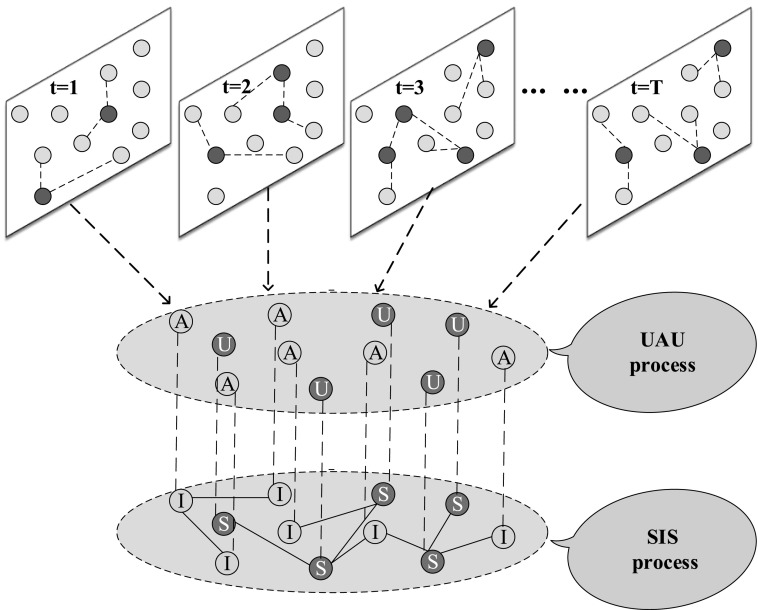
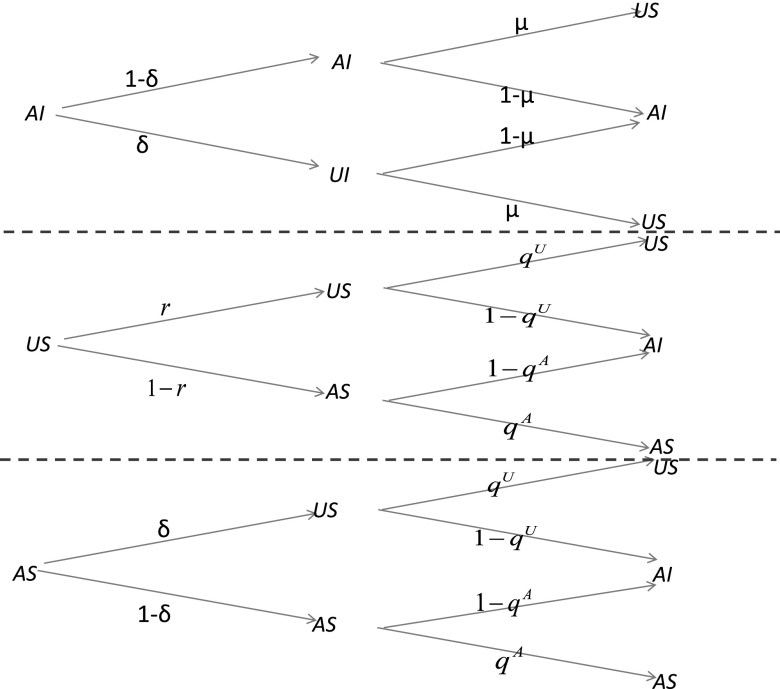
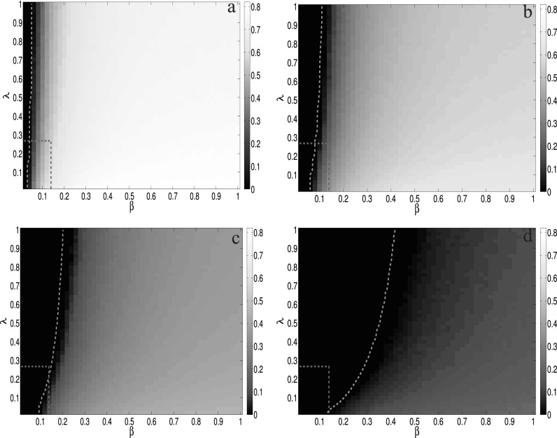
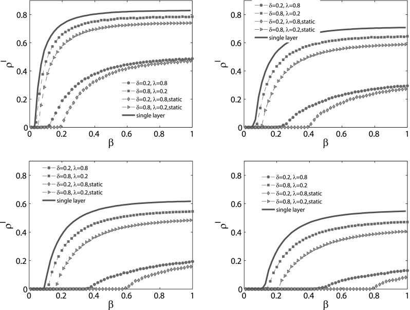
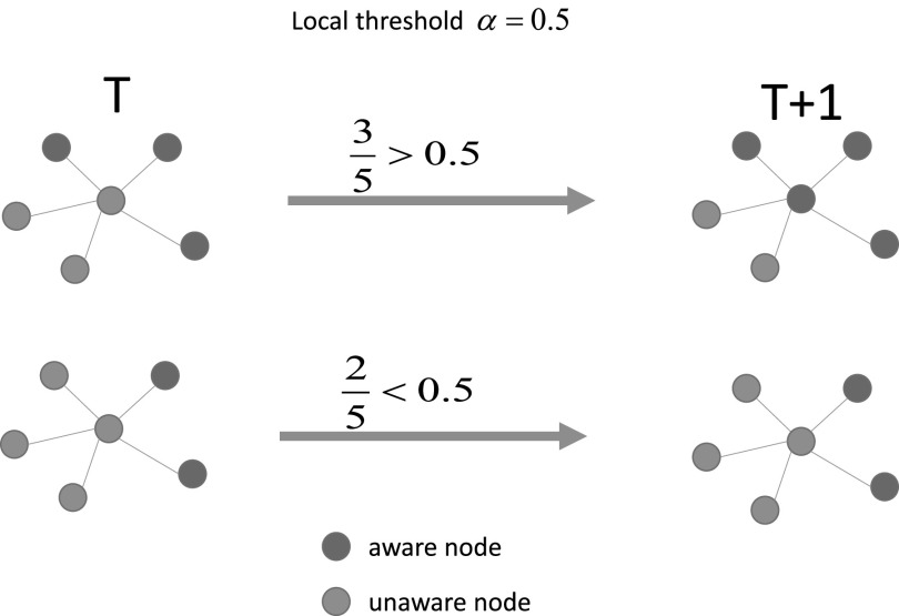
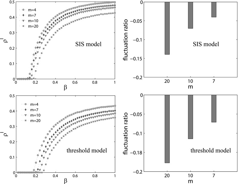
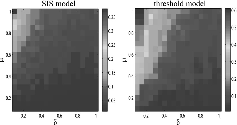
There has been growing interest in exploring the interplay between epidemic spreading with human response, since it is natural for people to take various measures when they become aware of epidemics. As a proper way to describe the multiple connections among people in reality, multiplex network, a set of nodes interacting through multiple sets of edges, has attracted much attention. In this paper, to explore the coupled dynamical processes, a multiplex network with two layers is built. Specifically, the information spreading layer is a time varying network generated by the activity driven model, while the contagion layer is a static network. We extend the microscopic Markov chain approach to derive the epidemic threshold of the model. Compared with extensive Monte Carlo simulations, the method shows high accuracy for the prediction of the epidemic threshold. Besides, taking different spreading models of awareness into consideration, we explored the interplay between epidemic spreading with awareness spreading. The results show that the awareness spreading can not only enhance the epidemic threshold but also reduce the prevalence of epidemics. When the spreading of awareness is defined as susceptible-infected-susceptible model, there exists a critical value where the dynamical process on the awareness layer can control the onset of epidemics; while if it is a threshold model, the epidemic threshold emerges an abrupt transition with the local awareness ratio α approximating 0.5. Moreover, we also find that temporal changes in the topology hinder the spread of awareness which directly affect the epidemic threshold, especially when the awareness layer is threshold model. Given that the threshold model is a widely used model for social contagion, this is an important and meaningful result. Our results could also lead to interesting future research about the different time-scales of structural changes in multiplex networks.

FIG. 1.

A simple example of the structure of the multiplex network proposed in the paper. The awareness layer is a time varying network where the spreading of awareness happens. At each time step, the topology structure of the awareness layer is built according to the activity driven model. Relying on the newly built network, the individuals interact with each other to change the states: unaware (green node) and aware (yellow node). The other layer corresponds to the network where epidemic transfers among two kinds of nodes, namely, susceptible (green node) and infected (red node). Individuals on two layers are the same. In particular, only three kinds of states exist in the multiplex network: unaware and susceptible, aware and infected, and aware and susceptible. Note that in the figure, red individuals on the time varying network represent the activated ones and each activated individual can have 2 connections with other individuals at each time step.

FIG. 2.

The probability tree for the transitions of states. The states include AI (aware and infected), US (unaware and susceptible), and AS (aware and susceptible). In the probability tree, μ represents transition probability from infected to susceptible, δ represents transition probability from aware to unaware. Meanwhile, q^A and q^U represent the transition probability for individual not being infected by neighbors if it is aware or unaware, respectively. r represents probability for unaware individual staying unaware. The coupled dynamical processes take place consecutive as time goes by.

FIG. 3.

The comparisons of the epidemic threshold between analytic results (MMCA method) and MC simulations as a function of the infected probability β and the aware probability λ. The green dashed line is the MMCA results for the epidemic threshold and the heatmap represents the density of infected nodes ρ^I obtained by MC simulations under different parameters. From top left to bottom right, the recovery rate μ and the forgetting rate δ are set to be (a) μ = 0.2, δ = 0.8, (b) μ = 0.4, δ = 0.6, (c) μ = 0.6, δ = 0.4, and (d) μ = 0.8, δ = 0.2, respectively. The dashed rectangle corresponds to the area where the metacritical points are located, which are bounded by the topological characteristics of each layer $\frac{1}{m(〈a〉+〈a^2〉)}$ and $\frac{1}{{\Lambda }_{\text{max}}(B)}$. The four phase diagrams are obtained by averaging 100 MC simulations for each point in the grid 50 × 50.

FIG. 4.

MC simulations for epidemic spreading on multiplex network (red lines) and single layer network (blue lines), as well as a two-layer static multiplex network (green lines). The topology structure of the single layer network is the same as the contagion layer of the multiplex network defined above. As for the static network, except that the awareness layer is a static network, its topology structure is totally the same as that of the time-varying network. On each panel, according to different values of the aware probability λ and the forgetting rate δ, we plot four dashed lines for the coupled dynamical processes. The red circle and green diamond line are under the condition when δ = 0.2 and λ = 0.8, while for the red square and green triangle line, δ = 0.8 and λ = 0.2. As for the recovery rate μ, the value is set to be (a) μ = 0.2, (b) μ = 0.4, (c) μ = 0.6, and (d) μ = 0.8. Each line is obtained by averaging 50 independent MC simulations.

FIG. 5.

Illustration of the threshold model used to simulate the spreading of information. Only if the ratio between the number of aware neighbors and its degree larger than the threshold value α, the unaware individual can become aware. Here, in the toy model, the threshold is set to be 0.5. The red individuals are aware, while the blue ones are unaware.

FIG. 6.

The comparisons of the epidemic threshold between numerical results (MMCA method) and MC simulations as a function of the infected probability β and the local threshold α. The green dotted line corresponds to the epidemic thresholds calculated by the MMCA method, while the heatmap represents the density of the infected nodes ρ^I obtained by MC simulations under different parameters. From top left to bottom right, the recovery rate μ and the forgetting rate δ are set to be (a) μ = 0.2, δ = 0.8, (b) μ = 0.4, δ = 0.6, (c) μ = 0.6, δ = 0.4, and (d) μ = 0.8, δ = 0.2, respectively. The four phase diagrams are obtained by averaging 100 MC simulations for each point in the grid 50 × 50.

FIG. 7.

MC simulations for epidemic spreading on multiplex network (circle lines) and single layer network (blue lines), as well as a two-layer static multiplex network (square lines). The topology structure of the single layer network is the same as the contagion layer of the multiplex network defined above. As for the static network, except that the awareness layer is a static network, its topology structure is totally the same as the time-varying network. The recovery rate μ is set as follows: (a) $\mu =0.2$, (b) $\mu =0.4$, (c) $\mu =0.6$, and (d) $\mu =0.8$. In each panel, the dashed lines represent the condition when the forgetting rate $\delta =0.2$ and for the dotted lines, $\delta =0.8$. Besides, the awareness probability is set to be 0.2. Every line is obtained by averaging 100 MC simulations.

FIG. 8.

The comparison of the steady density of the infected nodes ${\rho }_i^I$ between MMCA method (triangles) and MC simulations (circles). Left panel is obtained under the SIS model, while right panel is obtained under the threshold model. The other parameters are set as follows: $\lambda =0.2,\alpha =0.2$. Each line of the MC simulations is obtained by averaging 100 independent experiments.

FIG. 9.

The effects of different time varying topologies on the spreading of epidemics under the SIS model and the threshold model. For each model, we plot four dotted lines through changing the parameter m, namely, 4, 7, 10, and 20, which can produce different time varying networks. The left two panels show the percent of the infected nodes ρ^I as a function of β. Meanwhile, the right panels correspond to the fluctuation ratio calculated by Eq. (11).

FIG. 10.

The phase space of μ and δ with color corresponding to the effect of λ (SIS model, left panel) or α (threshold model, right panel). The settings of the multiplex network are the same as those described in Fig. 3. Importantly, each panel is obtained by two steps: for each pair values of (μ, δ), first, we calculate the epidemic thresholds by letting λ (α) be 0.8 and 0.2, respectively. Then, the final value, which is shown on each panel, equals the epidemic threshold at λ = 0.8 (α = 0.2) minus the epidemic threshold at λ = 0.2 (α = 0.2).

References

1. Pastor-Satorras R. and Vespignani A., Phys. Rev. Lett. 86, 3200 (2001).10.1103/PhysRevLett.86.3200 - DOI - PubMed
1. Newman M. E. J., Phys. Rev. E 66, 016128 (2002).10.1103/PhysRevE.66.016128 - DOI - PubMed
1. Moreno Y., Pastor-Satorras R., and Vespignani A., Eur. Phys. J. B 26, 521 (2002).10.1140/epjb/e20020122 - DOI
1. Dezso Z. and Barabási A.-L., Phys. Rev. E 65, 055103 (2002).10.1103/PhysRevE.65.055103 - DOI - PubMed
1. Balcan D. and Vespignani A., Nat. Phys. 7, 581 (2011).10.1038/nphys1944 - DOI - PMC - PubMed
Publication types