Imaging whole-brain cytoarchitecture of mouse with MRI-based quantitative susceptibility mapping

Abstract

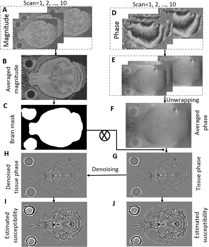
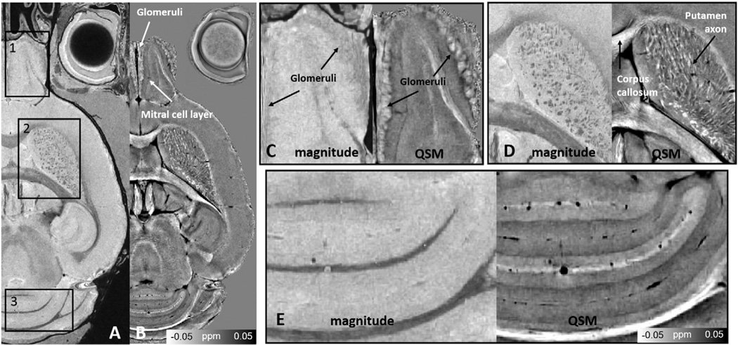
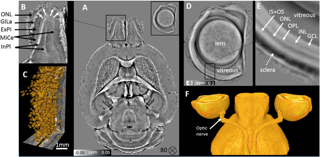
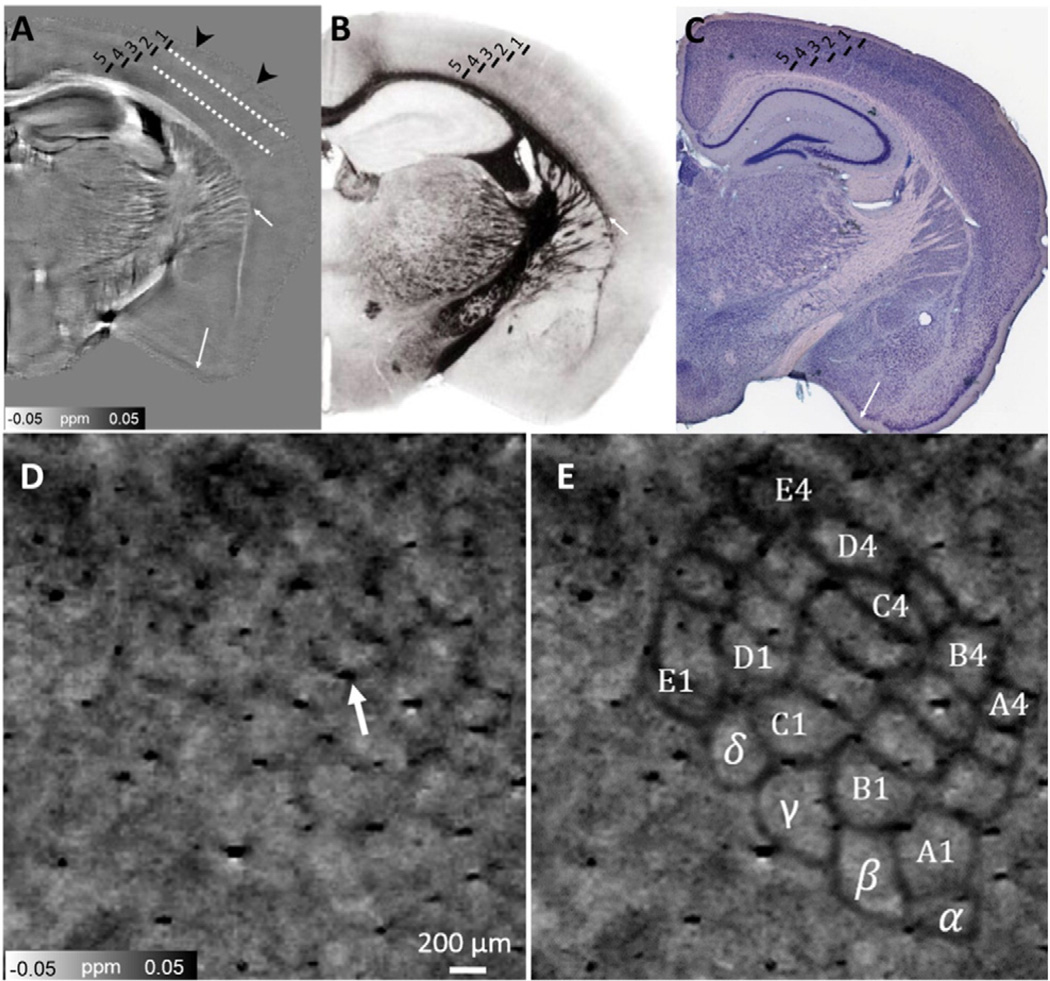
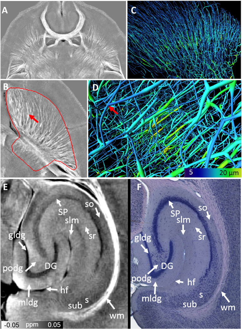
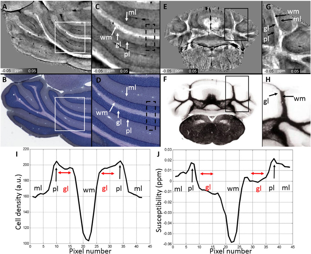
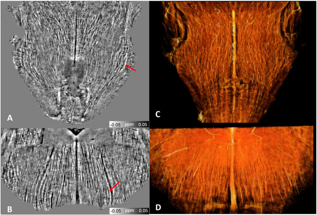
The proper microstructural arrangement of complex neural structures is essential for establishing the functional circuitry of the brain. We present an MRI method to resolve tissue microstructure and infer brain cytoarchitecture by mapping the magnetic susceptibility in the brain at high resolution. This is possible because of the heterogeneous magnetic susceptibility created by varying concentrations of lipids, proteins and irons from the cell membrane to cytoplasm. We demonstrate magnetic susceptibility maps at a nominal resolution of 10-μm isotropic, approaching the average cell size of a mouse brain. The maps reveal many detailed structures including the retina cell layers, olfactory sensory neurons, barrel cortex, cortical layers, axonal fibers in white and gray matter. Olfactory glomerulus density is calculated and structural connectivity is traced in the optic nerve, striatal neurons, and brainstem nerves. The method is robust and can be readily applied on MRI scanners at or above 7T.

Keywords: Cytoarchitecuture; Mouse brain; Quantitative susceptibility mapping.

Fig. 1

Schematic view of the data processing and QSM reconstruction. A: Magnitude images from multiple scans. B: Averaged magnitude image. C: Brain mask. D: Raw phase images from multiple scans. E: Unwrapped phase images. F: Averaged phase. G: Tissue phase obtained after removing background phase. H: Denoised tissue phase. I: QSM reconstructed using STARQSM. J: QSM reconstructed without phase denoising (G).

Fig. 2

Comparison between magnitude and QSM. A: Magnitude. B: QSM. QSM reveals additional anatomical detail in the olfactory bulb, corpus callosum, putamen, and cerebellum. Magnification of the areas outlined in black on the GRE magnitude and QSM are illustrated corresponding to (C) olfactory bulb, (D) striatum and (E) cerebellum.

Fig. 3

A: Susceptibility map shows olfactory bulb layers and retina layers. B: Magnification of the olfactory bulb in (A). GlLa: glomerular layer; ExPl: external plexiform layer; MiCe: mitral cell layer; InPl: internal plexiform layer. C: The glomeruli structure in the olfactory bulb represented by spherical volume. D: Susceptibility of the eye ball. E: Multiple distinct retinal layers (solid arrows) of alternating between bright and dark bands. GCL: ganglion cell layer; INL: inner nuclear layers; OPL: outer plexiform layer; ONL: outer nuclear layer; IS + OS: inner and outer photoreceptor segment. F: 3D volume rendering of the eye ball. It shows the optic nerve connecting the eye ball and the brain.

Fig. 4

Susceptibility map (A) of cortical layers and in comparison to myelin stained areas with different neuronal density (B) and a Giemsa stain containing different level of iron storage in the neuronal cell body (C). Fig. 4B has the author's permission to include myelin image 286 from Sidman, R.L., Kosaras, B., Misra, B.M. and Senft, S.L.: High Resolution Mouse Brain Atlas. 1999 (http://www.hms.harvard.edu/research/brain). Fig. 4C was reproduced with permission (http://brainmaps.org/ajax-viewer.php?datid=116&sname=3d2). Tangential view of the neuron somata in the vibrissal cortex revealed by magnetic susceptibility. D: QSM image revealed the distinct barrel structure arrangement. Individual barrels can be seen as diamagnetic areas while the boundaries (septa/wall) can be seen as paramagnetic areas. E: Manually drawn black lines indicate the individual barreloids within 24 barrel columns (α–δ, A1–A4). Arrow in Fig. 4D indicates the blood vessel in cortex.

Fig. 5

White matter and striatal tracts using QSM maps. A & B: Maximum intensity projection of QSM maps in the axial directions over 200 µm. C & D: Example of 3 dimensional reconstructed striatal tracts from magnetic susceptibility. E & F: Susceptibility map of hippocampus compared to a Giemsa stain at 0.46 µm/pixel resolution. SP: stratum pyramidale; DG: dentate gyrus; gldg: granule cell layer; hf: hippocampal fimbria; mldg: molecular layer; podg: polymorphic layer; s: subiculum; so: stratum oriens; sr: stratum radiatum; slm: stratum lacunosum-moleculare; subiculum (sub); wm: white matter. Giemsa staining figure was reproduced with permission (http://brainmaps.org/index.php?action=viewslides&datid=115).

Fig. 6

Susceptibility map of cerebellum (A, C, E & G) and comparison to a corresponding Giemsa stain (B & D) at 0.46 µm/pixel resolution and myelin stain (F & H). C and D are the zoomed images from the corresponding white boxes in A and B, respectively. Note that brighter white matter in C are diamagnetic and darker color in Giemsa stain in C & D indicates a denser cell body. G and H are the zoomed images from the corresponding black boxes in E and F, respectively. I and J are the averaged intensity values plotted along the vertical position within the dash line boxes in C and D, respectively. The profile in I is plotted from downsampled Giemsa stain by a factor of 20 to obtain the similar cell positions as those in susceptibility maps. gl: granular layer; ml: molecular layer; pl: Purkinje cell layer; wm: white matter. Fig. 6B & D was reproduced with permission (http://brainmaps.org/index.php?action=viewslides&datid=115). Fig. 6F was reproduced with author's permission from image 496 of Sidman, R.L., Kosaras, B., Misra, B.M. and Senft, S.L.: High Resolution Mouse Brain Atlas. 1999 (http://www.hms.harvard.edu/research/brain).

Fig. 7

Brainstem nerve tracts revealed by susceptibility maps (A & B) and 3D volume rendering (C & D).

References

1. Abduljalil AM, Schmalbrock P, Novak V, Chakeres DW. Enhanced gray and white matter contrast of phase susceptibility-weighted images in ultra-high-field magnetic resonance imaging. J. Magn. Reson. Imaging. 2003;18:284–290. - PubMed
1. Argyridis I, Li W, Johnson GA, Liu C. Quantitative magnetic susceptibility of the developing mouse brain reveals microstructural changes in the white matter. Neuroimage. 2014;88:134–142. - PMC - PubMed
1. Bagnato F, Hametner S, Yao B, van Gelderen P, Merkle H, Cantor FK, Lassmann H, Duyn JH. Tracking iron in multiple sclerosis: a combined imaging and histopathological study at 7 Tesla. Brain. 2011;134:3602–3615. - PMC - PubMed
1. Benner EJ, Luciano D, Jo R, Abdi K, Paez-Gonzalez P, Sheng H, Warner DS, Liu C, Eroglu C, Kuo CT. Protective astrogenesis from the SVZ niche after injury is controlled by Notch modulator Thbs4. Nature. 2013;497:369–373. - PMC - PubMed
1. Bilgic B, Pfefferbaum A, Rohlfing T, Sullivan EV, Adalsteinsson E. MRI estimates of brain iron concentration in normal aging using quantitative susceptibility mapping. Neuroimage. 2012;59:2625–2635. - PMC - PubMed