A population-based temporal logic gate for timing and recording chemical events

Abstract

Engineered bacterial sensors have potential applications in human health monitoring, environmental chemical detection, and materials biosynthesis. While such bacterial devices have long been engineered to differentiate between combinations of inputs, their potential to process signal timing and duration has been overlooked. In this work, we present a two-input temporal logic gate that can sense and record the order of the inputs, the timing between inputs, and the duration of input pulses. Our temporal logic gate design relies on unidirectional DNA recombination mediated by bacteriophage integrases to detect and encode sequences of input events. For an E. coli strain engineered to contain our temporal logic gate, we compare predictions of Markov model simulations with laboratory measurements of final population distributions for both step and pulse inputs. Although single cells were engineered to have digital outputs, stochastic noise created heterogeneous single-cell responses that translated into analog population responses. Furthermore, when single-cell genetic states were aggregated into population-level distributions, these distributions contained unique information not encoded in individual cells. Thus, final differentiated sub-populations could be used to deduce order, timing, and duration of transient chemical events.

Keywords: DNA memory; event detectors; integrases; population analysis; stochastic biomolecular models.

Figure 1. Design overview of a temporal logic gate

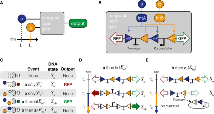
1. A temporal logic gate distinguishes between two chemical inputs (a, b) with different start times.

2. Implementation of the temporal logic gate using a set of two integrases with overlapping attachment sites. Chemical inputs a and b activate production of integrases intA and intB, which act upon a chromosomal DNA cassette.

3. Table with all possible inputs and outcomes to the event detector.

4. Sequence of DNA flipping following inputs with inducer a before inducer b (event E _ab).

5. Sequence of DNA flipping following inducer inputs with b first (event E _ba). In any events in which b precedes a, the unidirectionality of the intB attachment sites results in excision.

Figure 2. A Markov model of integrase‐mediated DNA flipping

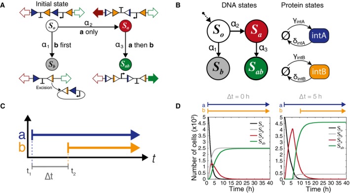
1. The four possible DNA states, illustrated with DNA state diagrams. All DNA begins in the initial state S _o, and there are no reverse processes. The propensity functions α₁, α₂, and α₃ are dependent on the concentration of the two integrases and correspond to the events b first (E _b), a only (E _a), and a then b (E _ab), respectively.

2. Representation of the same model as a Markov chain. Integrases are represented simply as protein states with production (γ_A; γ_B) and degradation (δ_A; δ_B) rates.

3. Graphical representation of inducer step functions. ∆t is defined as difference between the start time of the first inducer and start time of the second.

4. Simulation results for inducer separation times of 0 and 5 h. There are four possible DNA states, but all cells end up in either the S _b or S _ab final states. Individual trajectories are simulated for 5,000 cells and the number of cells in each DNA state is summed for each time point (Appendix Fig S2).

Figure 3. Simulation results for inducer separation time for ∆t = 0–10 h

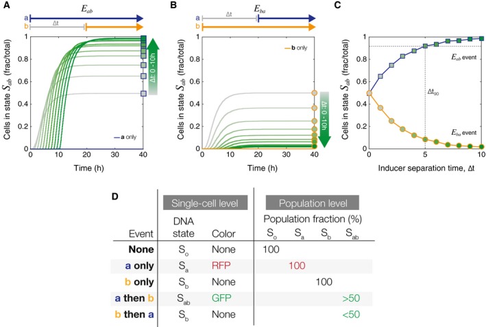
1. The population fraction (N/5,000 cells) that switches into state S _ab following an E _ab event is dependent on the inducer separation time, ∆t. The gray to dark green color gradient represents increasing ∆t values. Square markers indicate final population fractions for specific values of ∆t.

2. In the case of the inverse E _ba event, the fraction of cells in state S _ab decreases monotonically with increasing ∆t. Circular markers indicate final population fractions for specific values of ∆t.

3. Final S _ab cell fractions from (A, B) are plotted as a function of ∆t. Blue line with square markers shows end point population fractions from an E _ab event. Yellow line with circular markers shows final end point population fractions from an E _ba event. The gradient inside the markers corresponds to increasing ∆t value. The dotted gray line corresponds to the ∆t ₉₀, the value of ∆t at which ≥ 90% of the cells are in state S _ab. All simulations were done with a population of N = 5,000 cells.

4. Chart showing differences in information that can be recorded at the single‐cell versus the population level. In particular, E _ba does not have a unique single‐cell genetic state, but has a clear distinct population‐level phenotype.

Figure 4. In vivo results for varying inducer separation time from ∆t = 0–8 h

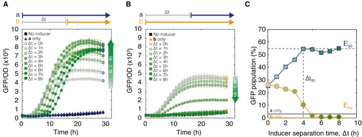
1. Populations of cells exposed to an E _ab event sequence. Cell switching to state S _ab (indicated by GFP fluorescence) begins when inducer b (aTc) is added. Maximum normalized GFP fluorescence increases as a function of the inducer separation time ∆t. Gray to dark green gradient represents increasing ∆t values. Square markers are final end point measurements. Error bars represent standard error of the mean.

2. Cells exposed to the inverse E _ba sequence of events. GFP fluorescence decreases monotonically with increasing inducer separation time between b and a. Circular markers are final end point measurements.

3. Final population distributions from (A, B) at 30 h are plotted as a function of ∆t. Cells were gated by GFP fluorescence to identify percentage of S _ab cells. Dotted line marks ∆t ₉₀ detection limit.

Source data are available online for this figure.

Figure EV1. Flow cytometry data for varying inducer separation time from ∆t = 0 to 8 h (~10⁶ cells per population)

The populations are gated by fluorescence into Q1 (S _ab, GFP only), Q2 (S _ab, RFP and GFP), Q3 (S _a, RFP only), and Q4 (S _o, S _b, non‐fluorescent). There is a transitory phase (Q2) in which cells contain both GFP and RFP. This is due to slow dilution of RFP through cell division even after cells have switched to S _ab and begun production of GFP. Cells in Q1 + Q2 are used for the final GFP population fractions in Fig 4C.

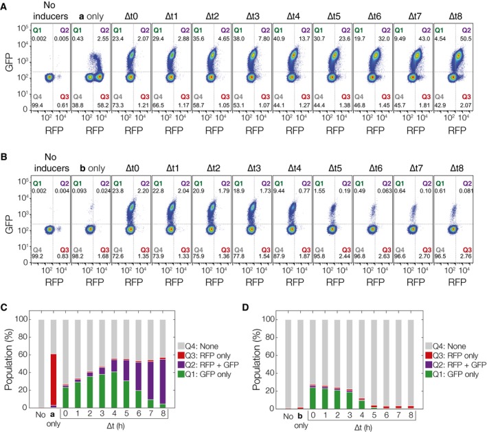
1. E _ab cell populations plotted by their RFP and GFP expression with increasing ∆t. Leaky expression of PBAD‐intA can be estimated by looking at Q3 of the No inducers,b only populations (˜0.5–2%). Leaky expression of Ptet‐intB can be estimated with Q1 + Q2 fractions of the a only population (˜2–3%).

2. E _ba populations with increasing ∆t.

3. Population fractions by quadrant for a then b, E _ab.

4. Population fractions by quadrant for b then a, E _ba. Individual flow cytometry histograms can be found in Appendix Figs S8–S10.

Source data are available online for this figure.

Figure 5. Varying model parameters for integrase flipping and leaky expression

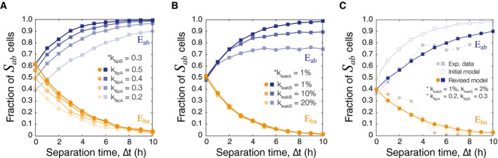
1. As DNA flipping rates of intA ($k_{flipA}$) are decreased relative to $k_{flipB}$, the population of S _ab cells at ∆t = 0 h has a downward shift. Simulations are done with N = 3,000 trajectories/marker.

2. Increasing the leaky expression of intB ($k_{leakB}$) changes the maximum threshold of cells that correctly identify S _ab even at high ∆t. Leakiness is defined as a percentage of the induced integrase production rate ($k_{prod\ast }$).

3. The model was revised to more closely match the experimental data by constraining parameters for leaky expression and varying integrase flipping (N = 5,000). Mean squared error was calculated between the experimental data and the initial and revised models to find an optimized pair of $k_{flipA,B}$ values (Appendix Fig S13). The revised parameters are k _flipA = 0.2 h⁻¹, k _flipB = 0.3 h⁻¹, k _leakA = 1% of k _prodA(μm³ · h)⁻¹, and k _leakB = 2% of k _prodB(μm³ · h)⁻¹.

Figure 6. Simulation results for pulse width modulation

Simulations were done with revised parameters found in Fig 5C.

1. Inducer a can be used as a reference signal against which to measure the time and duration of the inducer b pulse.

2. The population eventually divides into one of two sub‐populations: those that see inducer a first and those that see inducer b first. Only if a cell has entered the a first pathway does it have the possibility to express RFP or GFP. Furthermore, S _a can be thought of as a necessary precursor to S _ab.

3. A matrix illustrating a subset of the ∆t and PW _b values to be tested.

4. Simulation results show that for any given ∆t, the number of cells in S _b = (total number of cells − (S _a + S _ab))

5. The fraction of the population in the S _a state is totally independent of ∆t and depends only on the pulse duration of inducer b.

6. Once PW _b is known, then the fraction of the population in S _ab state can be used to find the time at which the pulse of inducer b began. N = 3,000 cell trajectories for each value of ∆t, PW _b.

Figure 7. Determining arrival time and pulse duration of inducer b with population fractions

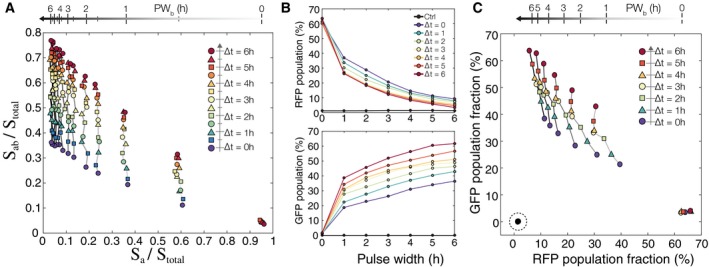
1. Simulation results from testing an 11 × 11 matrix of parameters with ∆t and PW _b varying from 0 to 6 h in increments of 0.5 h. Each point represents a population of 3,000 cells. Increasing PW _b goes from right to left, and increasing ∆t goes from bottom to top.

2. Experimental results showing RFP and GFP population fractions as a function of increasing ∆t and PW _b. Experimental results were obtained by exposing temporal logic gate E. coli populations to varying PW _b and ∆t values (0–6 h, 0.01%/vol L‐ara, 200 ng/ml aTc, measurements taken at 48 h).

3. A scatterplot of each population using their RFP and GFP fractions as coordinates (˜10⁶ cells per population). The non‐induced control samples are indicated with a dotted circle on the bottom left, and the samples with PW _b = 0 h are on the bottom right. Samples with the same PW _b are connected with a solid line, and line darkness represents increasing PW _b duration. Samples with the same ∆t are shown with the same colored shape marker and increasing ∆t goes from bottom to top.

Source data are available online for this figure.

Figure EV2. Selected flow cytometry panels for Fig 7C populations

Cell populations are gated by RFP and GFP fluorescence into quadrants Q1 (S _ab, GFP only), Q2 (S _ab, RFP and GFP), Q3 (S _a, RFP only), and Q4 (S _o, S _b, non‐fluorescent). Percentage of total cells in each quadrant is shown under the quadrant label in each panel.

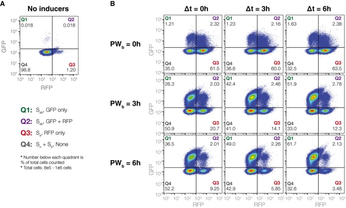
1. Control population not exposed to any inducers. There is minimal leaky expression (1–2%) into Q3 after 36 h of growth.

2. Populations for PW _b and ∆t values of 0, 3, and 6 h. For PW _b = 0 h populations, ˜60% of the cells switch to S _a (Q3), with ˜3% intB leaky expression going into Q1 and Q2. As PW _b increases, the S _a fraction drops from 60% (PW _b = 0 h) to 10–20% (PW _b = 3 h) to less than 10% (PW _b = 6 h). As ∆t increases, the percentage of cells in S _ab (Q1) increases from 20–40% (∆t = 0 h) to 40–50% (∆t = 3 h) to 50–60% (∆t = 6 h). S _a populations (Q3) also drift downwards with increasing ∆t, rather than staying constant as predicted in simulation. Lower ∆t results in higher S _b populations, which, combined with S _o cells, make up Q4. Critically, the percentage of the population expressing both RFP and GFP simultaneously (Q2) is always < 3%. This ensures that RFP is a reliable determinant of S _a state cells, and subsequently, of PW _b.

Source data are available online for this figure.

Figure 8. Determining prediction resolution for PW _b and ∆t from population data

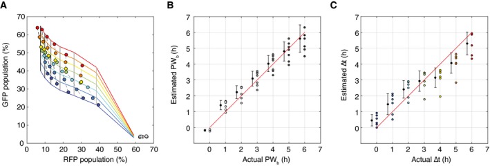
1. A mesh generated from fitted curves for PW _b as a function of RFP population percentage(R) and ∆t as a function of pulse width and GFP population percentage(G). Experimental data are overlaid.

2. Comparison of actual versus estimated PW _b values generated by fitted function PW _b(R). For each actual PW _b value, the average of the estimated PW _b values with ± 1 standard deviation (slightly offset on the x‐axis for better comparison).

3. Comparison of actual versus estimated ∆t generated by the fitted function ∆t(G; PW _b). For each actual ∆t value, the average of the estimated ∆t with ± 1 standard deviation (slightly offset on the x‐axis for better comparison).

Source data are available online for this figure.