. 2016 Mar;3(1):011105.
doi: 10.1063/1.4941675. Epub 2016 Mar 10.

Optical tracking of nanoscale particles in microscale environments

Affiliations

Optical tracking of nanoscale particles in microscale environments

P P Mathai et al. Appl Phys Rev. 2016 Mar.

Abstract

The trajectories of nanoscale particles through microscale environments record useful information about both the particles and the environments. Optical microscopes provide efficient access to this information through measurements of light in the far field from nanoparticles. Such measurements necessarily involve trade-offs in tracking capabilities. This article presents a measurement framework, based on information theory, that facilitates a more systematic understanding of such trade-offs to rationally design tracking systems for diverse applications. This framework includes the degrees of freedom of optical microscopes, which determine the limitations of tracking measurements in theory. In the laboratory, tracking systems are assemblies of sources and sensors, optics and stages, and nanoparticle emitters. The combined characteristics of such systems determine the limitations of tracking measurements in practice. This article reviews this tracking hardware with a focus on the essential functions of nanoparticles as optical emitters and microenvironmental probes. Within these theoretical and practical limitations, experimentalists have implemented a variety of tracking systems with different capabilities. This article reviews a selection of apparatuses and techniques for tracking multiple and single particles by tuning illumination and detection, and by using feedback and confinement to improve the measurements. Prior information is also useful in many tracking systems and measurements, which apply across a broad spectrum of science and technology. In the context of the framework and review of apparatuses and techniques, this article reviews a selection of applications, with particle diffusion serving as a prelude to tracking measurements in biological, fluid, and material systems, fabrication and assembly processes, and engineered devices. In so doing, this review identifies trends and gaps in particle tracking that might influence future research.
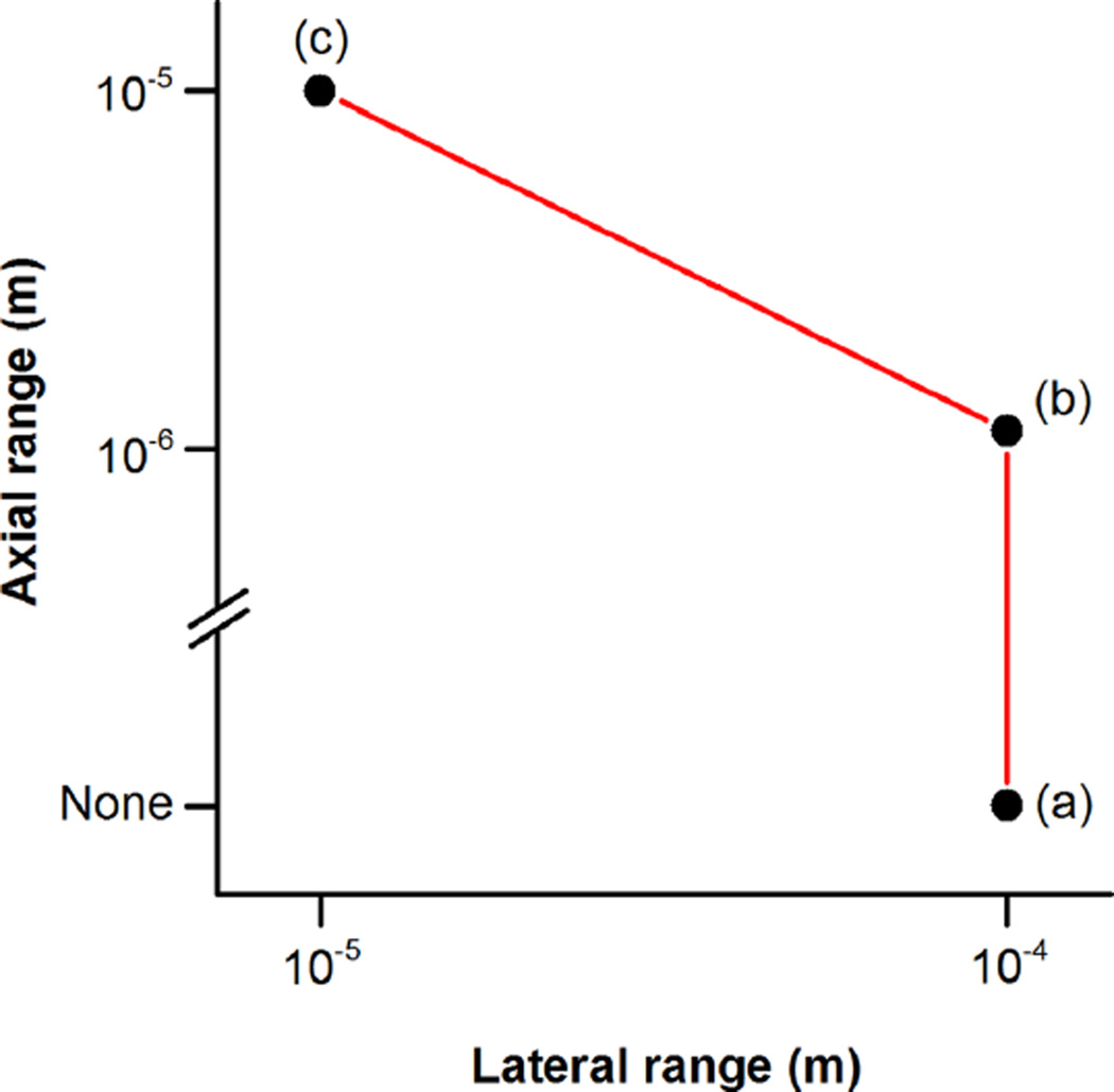

Figures

FIG. 1
FIG. 1
A map serving as an initial guide to the optical tracking of nanoscale particles in microscale environments. Horizontal and vertical axes, in units of meters and seconds, respectively, denote various scales of length and time that are relevant to some of the applications, hardware, and processes that this article reviews. Red data markers with parenthetical letters indicate specific applications, with the horizontal axis denoting the reported spatial precision and the vertical axis denoting the inverse of the reported temporal bandwidth. The values of temporal bandwidth correspond to (a)–(e) the times to update a sensor for tracking single particles and (f)–(h) the times to acquire a series of images for tracking multiple particles. Applications of particle tracking are remarkably diverse. (a) Ballistic-to-diffusive transition of a particle in a fluid. (b) Viscoelastic response of diluted polyethylene oxide. (c) Dynamics of unbound myosin head. (d) Hop–diffusion of lipid in cell membrane. (e) Kilohertz rotation of nanorods propelled by ultrasound. (f) Mapping structural heterogeneity of a polymer film. (g) Highest temporal bandwidth for photoactivated localization microscopy in three dimensions. (h) Chromosome motion during cell division. Red line segments perpendicular to axes indicate specifications of common hardware for nanoparticle tracking. Red line segments, rays, and lines along axes indicate spatial or temporal ranges of interest. Visible and near-infrared (vis–NIR) wavelengths range between 0.4 µm and 1 µm. The localization precision of an isolated isotropic emitter extends down from approximately 200 nm to below 1 nm. The conformations of proteins involve dynamics at time scales between 100ns and 1ms. The red line within the white space of the figure indicates the Stokes-Einstein estimate for the mean squared displacement in one dimension of a nanoparticle diffusing freely in water at an absolute temperature of 300 K. Any point on this line corresponds to the time for diffusion to displace the particle by a length equal to the diameter of the particle. Transitions from diffusive to ballistic motion occur at shorter scales of length and time, depending on the properties of the particle and fluid, and deviate from this line.
FIG. 2
FIG. 2
A simulation estimating the irradiance necessary to localize a static fluorescent bead to a target precision, as well as the motion blur of a diffusing bead, both varying as a function of time. Eq. (4) relates the irradiance P/Aillum to the integration time t to achieve a static lateral localization precision of 10 nm, with parameter values c = 3 × 10⁸ m · s−1, NP = 350, λ = 600 nm, σem= 690 nm2, Y = 0.92, ηQE = 0.7, and s = 0.067 corresponding to an objective lens having NA = 0.5 that is immersed in air. The motion blur in one dimension due to diffusion is 2Dt, where D ≈ 4 µm2 · s−1 is the diffusion coefficient of a spherical bead with radius R = 50 nm in water at an absolute temperature of 300 K. With all other parameters held constant, the irradiance needed to localize a particle to a target precision varies as R−3 while the motion blur varies as R−1/2.
FIG. 3
FIG. 3
A schematic classifying apparatuses and techniques by the number of light sensors arrayed and the resulting number of particles tracked. (a) and (b) A EMCCD or CMOS digital camera uses an array of many light sensors for widefield imaging, which enables simultaneous measurement of many nanoparticles. This schematic assumes an image pixel size of 100nm, with each nanoparticle requiring an area of 1 µm × 1 µm for the image of the nanoparticle to not spatially overlap with the images of other nanoparticles. (c) These values set a conservative lower limit of 102 light sensors to localize each nanoparticle. Such an apparatus tends towards two-dimensional measurements and can integrate optical elements to enable three-dimensional imaging capability. The information content can be higher due to the large number of light sensors, within the constraints of signal-to-noise ratio. Assuming 103 incident photons on the sensor array having the above parameter values, a mean value of 10 photons is incident on each pixel, for which modern EMCCD and sCMOS cameras have signal-to-noise ratio >2 per pixel. (d) A point sensor, such as an avalanche photodiode, can be combined with other optical, mechanical, and electrical hardware to track single particles over wide lateral and axial ranges, trading off other degrees of freedom to do so. Such an apparatus necessarily involves feedback control to actively track the particle, with information from the light sensor being combined with information from the other hardware in the tracking system.
FIG. 4
FIG. 4
A simulation comparing three microscopy techniques shows differences in the localization precision that is theoretically achievable. Contour plots show cross sections of the logarithm of the normalized intensity distribution of a point particle that emits light isotropically at the focus of (a) conventional, unaberrated, (b) confocal, two-photon, and (c) 4Pi, Type C microscopes. The intensity distributions, which are symmetric about the optical axis in each case, are normalized relative to the respective central maxima, with the smallest pseudo-elliptical contours enclosing these maxima having equal log normalized intensities. The decreasing area that these central contours enclose, from (a) to (c), indicates the increasing intensity gradient and improving localization precision that is theoretically achievable. For all simulations, the emission wavelength of the point particle in vacuum is λ = 482 nm and the numerical aperture of all objective lenses is 1.27. In the following comparison of simulation results, the variable z denotes the axial coordinate and the variable r denotes the lateral coordinate. The function h(r, z) denotes the amplitude of the detected intensity at (r,z) of the conventional, unaberrated microscope, which serves as a reference for the comparison. Simulated intensities at (r, z) for the three cases differ as follows. (a) The image intensity for the conventional, unaberrated microscope is h2(r, z). The intensity decays more gradually in the axial direction than the lateral direction, making axial localization less precise than lateral localization. (b) For the confocal two-photon microscope, the simulated intensity is h4(r/2, z/2) · h2(r, z). The simulation assumes an excitation wavelength of 2λ, so a factor of 1/2 scales the coordinates in the quartic term, with the fourth power stemming from the joint probability of two photons exciting the point particle. The decay of intensity in this case is sharper than the conventional, unaberrated microscope along both coordinates. (c) A 4Pi Type C microscope uses two objective lenses, both to excite the point particle and to collect the emitted signal. This simulation assumes that the excitation and emission wavelengths are equal. Two beams passing through the objective lenses interfere constructively at focus. Light emitted from the point particle forms a constructive interference pattern at the plane of the imaging sensor. With these assumptions, the intensity simulated for this case is |h(r, z) + h(r, −z)|4. Though the intensity decay near the central spot in this case is sharper than the other two cases due to the intended interference, the imaging sensor also detects a set of side lobes for the same reason. A mathematical deconvolution of these lobes is necessary to localize the point particle using Gaussian centroiding.
FIG. 5
FIG. 5
A schematic showing that apparatuses and techniques using imaging sensors typically provide more lateral range than axial range. (a) At focus, the image from a conventional microscope provides no localization precision out of the image plane due to the near symmetry of the point spread function in the axial direction. (b) Astigmatic modification of the point spread function with a cylindrical lens increases axial range without reducing the lateral range. (c) A microscope with diffractive optical elements simultaneously images multiple focal planes across the sensor array, reducing lateral range and increasing axial range for a fixed localization precision.
FIG. 6
FIG. 6
A schematic showing how systems for tracking single particles can combine moving parts or confining devices with a small number of light sensors. (a) A piezoelectric stage provides nanometer resolution and kilohertz bandwidth, relying on a light sensor and feedback control for guidance. (b) A tracking system combines a piezoelectric actuator guiding an illumination volume and an EMCCD camera with a region of interest of tens of pixels to track fluorescent beads in three dimensions. (c) A technique combines a nanofluidic channel with a sequential pair of illumination volumes and avalanche photodiodes to track and superresolve fluorescent DNA molecules in one dimension. (d) A single avalanche photodiode senses light at the nanosecond scale of the lifetime of an organic fluorophore, relying on a piezoelectric actuator for spatial information.

References

    1. Toschi F, Bodenschatz E. Annu. Rev. Fluid Mechan. 2009;41:375–404.
    1. Chen Q, Cho H, Manthiram K, Yoshida M, Ye X, Alivisatos AP. ACS Cent. Sci. 2015;1:33–39. - PMC - PubMed
    1. Manzo C, Garcia-Parajo MF. Rep. Prog. Phys. 2015;78(12):124601. - PubMed
    1. Backlund MP, Lew MD, Backer AS, Sahl SJ, Moerner WE. ChemPhysChem. 2014;15:587–599. - PMC - PubMed
    1. Kheifets S, Simha A, Melin K, Li T, Raizen MG. Science. 2014;343(6178):1493–1496. - PubMed

LinkOut - more resources