Analysis of complex neural circuits with nonlinear multidimensional hidden state models

Abstract

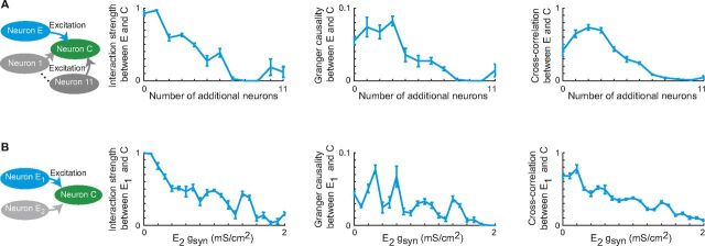
A universal need in understanding complex networks is the identification of individual information channels and their mutual interactions under different conditions. In neuroscience, our premier example, networks made up of billions of nodes dynamically interact to bring about thought and action. Granger causality is a powerful tool for identifying linear interactions, but handling nonlinear interactions remains an unmet challenge. We present a nonlinear multidimensional hidden state (NMHS) approach that achieves interaction strength analysis and decoding of networks with nonlinear interactions by including latent state variables for each node in the network. We compare NMHS to Granger causality in analyzing neural circuit recordings and simulations, improvised music, and sociodemographic data. We conclude that NMHS significantly extends the scope of analyses of multidimensional, nonlinear networks, notably in coping with the complexity of the brain.

Keywords: causal analysis; decoding; functional connectivity; hidden Markov models; machine learning.

Fig. 1.

Description of the NMHS model. (A) Schematic diagram of a neuronal microcircuit with an extraneous neuron. An ideal interaction detection algorithm would identify and characterize the interactions among all neurons in the microcircuit, and identify the extraneous neuron as unconnected. (B) Each state describes a probability distribution of observed outputs. (C) The transitions of a process depend on the state of its neighbors, such that process B will undergo transitions (light blue or light red) corresponding to the current state of process A (dark blue or dark red). (D) At a given time, t, the output of a process depends solely on the state of that process, and the transitions of that process depend on both its current state and the states of its neighbors. (E) Flowchart of the NMHS method. We search for a model that optimizes the likelihood of the data. We conclude that there is an interaction between A and B if the likelihood of our optimized NMHS model is greater than the likelihood of an unconnected model. By analyzing the transition and emission matrices, we can characterize the strength of the interactions and decode the behavior of A and B. (F) When the state of one process affects the transition behavior of another process, the two processes are interacting. The more the transitions of the process are affected, the stronger the interaction.

Fig. S1.

Application of the model to different interaction scenarios. (A) A two-state NMHS model in which Neuron A affects Neuron B, but Neuron B does not affect Neuron A, i.e., a “unidirectional interaction” model. Note that when Neuron B changes state, Neuron A’s behavior is unaffected (TA,I = TA,II), but when Neuron A changes state, the behavior of Neuron B will change (TB,1 ≠ TB,2). (B) An NMHS model with no interactions. (C) A bidirectional model in which both neurons affect the behavior of the other. (D) Graphical representation of how the NMHS model evolves over time. Arrows represent causal interactions. State transitions can be affected by all neurons, but emissions are only affected by the current state of a neuron. (E) To determine the optimal threshold multiplier for selecting a interacting vs. noninteracting model, we compute a receiver operating characteristic curve using a simulation that is similar to the dataset of interest by plotting the detection rate against the false positive rate for a range of possible multipliers. (F) For each of six different simulated common-cause networks with varying interaction strengths, we train five different models. With an appropriate choice of threshold, we see that the weakly interacting networks are better explained by a noninteracting model, but strongly interacting networks are better explained by a model with a high total interaction strength. (G) Multiple models may sometimes explain the data equally well, as shown here with a common cause model. In this case, decoding and interaction strength estimation cannot proceed, but total interaction detection is not affected. (H) Detailed view of the five trained models from the common-cause network in G, with simulated interaction strength of 0.6. We see that all five models, although are different, have similar total interaction strengths.

Fig. 2.

Verification of interactivity and decoding on neuronal microcircuits. (A) We first identified putative microcircuits: sets of two or three neurons such that the neurons are responders to stimulation of counterpart regions. (B) An example of a responding neuron, recorded in the DMS. In the raster plot (Left) and histogram (Right), spikes of the DMS neuron are aligned to stimulation of the PFC at time 0. (C) We recorded the activity of these putative microcircuits of neurons as a rat performed a decision-making task ( Supporting Information ). (D) We evaluated the ability of NMHS (Left) and GC (Right) to detect interactions in putative microcircuits. Microcircuits are categorized as bidirectional responders (both neurons respond to stimulus), unidirectional responders (one neuron responds to stimulus), unconnected (two recordings taken from different sessions, aligned to task events), or shuffled (recordings from connected circuits with observations shuffled over time). Cross-correlation analysis is shown in Fig. S2D . (E) The same evaluation, on microcircuits of three neurons (see also Fig. S2E ). (F) NMHS is also a valuable tool for decoding neuronal microcircuits. In an illustration with task recordings, NMHS and HMM find neuron hidden states with high (red), middle (yellow), or low (blue) activity in the SNpc (Left), DMS (Center), and PFC (Right) during the task. In hidden state plots, trials (horizontally stacked) are aligned to trial start, and black squares indicate the turn onset.

Fig. S2.

Preprocessing and decoding of neuronal data. (A) Bin size optimization for the LFP analysis shown in C. NMHS interactivity is calculated for many bin sizes, and the bin size that produces maximum interactivity is identified. (B) Dependence of false positive rate and detection rate on bin size. (C) An example of preprocessing LFP recordings for analysis by NMHS. In this example, recordings were binned into 59-ms intervals (vertical lines), and mean activity in each bin (green dots) was categorized by quartile (black horizontal lines). (D) Cross-correlation for the dataset plotted in Fig. 2D . (E) Cross-correlation for the dataset plotted in Fig. 2E . (F) Application of NMHS for the LPF analysis shown in A and B. In the hidden state plots, states (red: higher activity state, blue: lower activity state) of the motor cortex (Upper) and anterior caudate nucleus (Lower) are aligned to state transitions in the putamen (time 0). Hidden states in the motor cortex preceded the hidden states in the putamen by 50 ms, and there was no observed relation between the anterior caudate nucleus and putamen.

Fig. 3.

Validation on simulated microcircuits. (A–D) Simulation data were generated from two-node, two-state, three-emission NMHS matrix models (A). Interactivity estimated using NMHS (B), GC (C), and cross-correlation (D) was plotted against the simulated interactivity. (Blue points represent how much node 2 is affected by node 1; red vice versa.) (E–H) A Hodgkin–Huxley model simulates a triplet of neurons with two excitatory synapses (E). The strength of each interaction in the triplet is estimated using NMHS (F), GC (G), and cross-correlation (H) and plotted against the simulated synaptic strength (g_syn). The remaining interactivity directions are shown in Fig. S3E . (I–L) Interactivity of a similar Hodgkin–Huxley model with one excitatory and one inhibitory synapse (I), estimated with NMHS (J), GC (K), and cross-correlation (L) (see also Fig. S3F ).

Fig. S3.

Additional comparisons of performance of NHMS, GC, and cross-correlation on simulated microcircuits. (A) Estimated interactivity plotted as a function of simulated interactivity in a three-node matrix model calculated with NHMS (Left), GC (Center), and cross-correlation (Right). Simulated interactivity was varied by adding noise of various magnitudes to a baseline model described by transition and emission matrices. (B) Estimated interactivity as a function of simulated synaptic strength in a two-neuron model with an excitatory synapse. Data were generated using a Hodgkin–Huxley model where an upstream neuron synapses onto a downstream neuron. We varied the g _syn parameter, which corresponds to simulated synaptic strength. The downstream neuron does not synapse onto the upstream neuron. Line colors represent the direction of estimated interactivity. (C) Estimated interactivity in a two-neuron model with an inhibitory synapse. (D) Estimated interactivity in a two-neuron model with an excitatory synapse that provides an oscillatory input. (E) Estimated interactivity of the remaining four potential interactions of the three-neuron model with two excitatory inputs shown in Fig. 3 E–H (only one interaction for cross-correlation). All four interactions have low interactivity values, as expected, because there is no simulated interaction between them. (F) Estimated interactivity of the remaining potential interactions of the model shown in Fig. 3 I–L .

Fig. S4.

Detecting interaction strength in simulated circuits of Hodgkin–Huxley neurons. (A) Simulation of a multineuron network using a Hodgkin–Huxley model. We measure the interactivity from Neuron E to Neuron C (with a fixed simulated synaptic strength of g _syn = 0.4), while increasing the number of unmeasured neurons in the network (Neurons 1–11, each with a synaptic strength of g _syn = 0.2). We see that NMHS, GC, and cross-correlation all demonstrate a decreasing value with an increasing number of unmeasured neurons, because the activity of Neuron C is influenced more strongly by the unmeasured activity. (B) A similar simulation of a three-neuron network, keeping the synaptic strength of the measured pair (Neuron E₁ and Neuron C) constant (g _syn = 0.5), while increasing the synaptic strength between the unmeasured pair (Neuron E₂ and Neuron C).

Fig. 4.

Application to musical improvisation recordings and static data. (A) We collected recordings, in separate channels, of three guitarists improvising classic rock music. (B) NMHS determined interaction between three voices of a single band (coimprovised), three voices from separate bands (separately improvised), and randomly permuted recordings of three voices from a single band (shuffled). (C) NMHS attributed different interactivity from improvisation leaders to followers, from followers to leaders, and between followers. (D) Interaction strength detected by NMHS in the analysis of the activity of only three guitarists out of a larger group of three to six musicians. (E) In an application on a static network, NMHS analyzed sociodemographic data. In this static model, individuals in strata (boxes) are assigned states (blue and red ovals) that describe their wealth and education. (F) NMHS found interactivity between sociodemographic strata. (G) A probabilistic XOR model, where the output is produced by applying an XOR rule to a bin in the input streams with a set probability P. If the XOR rule is not applied, the output value is selected randomly. (H) NMHS performance in detecting interactivity strength between the input streams as a function of increasing P. (I) Cross-correlation performance in detecting the same interaction.

Fig. S5.

Preprocessing, interactivity, and decoding of musical improvisation recordings. (A) Pitch classifier used for extracting notes from guitar recordings shown in Fig. 4A . (B) Dependence of false positive rate and detection rate on bin size. (C) Cross-correlation of the dataset plotted in Fig. 4B . (D) NMHS was tested by comparing total interactivity in mixed groups with two voices (one band and one voice from a separate band) and in groups of two and three voices from a three-guitarist band. (E) NMHS assigns hidden states (red, higher activity state; blue, lower activity state) to the guitar recordings, which correlated with the pitches played by the improvisers. Recordings of the follower voices were aligned to state changes of the leader (time 0). The hidden state plot indicates that a band is synchronized with a short time delay and that we can identify the strategy of the followers (mimicking or contrasting) based on their hidden states.

References

1. Granger CWJ. Investigating causal relations by econometric models and cross-spectral methods. Econometrica. 1969;37(3):424–438.
1. Putnam RD. Our Kids: The American Dream in Crisis. Simon and Schuster; New York: 2015.
1. Sugihara G, et al. Detecting causality in complex ecosystems. Science. 2012;338(6106):496–500. - PubMed
1. Kispersky T, Gutierrez GJ, Marder E. Functional connectivity in a rhythmic inhibitory circuit using Granger causality. Neural Syst Circuits. 2011;1(1):9. - PMC - PubMed
1. Oweiss KG. Statistical Signal Processing for Neuroscience and Neurotechnology. Academic; Cambridge, MA: 2010.
Publication types
LinkOut - more resources