Simulation of Code Spectrum and Code Flow of Cultured Neuronal Networks

Abstract

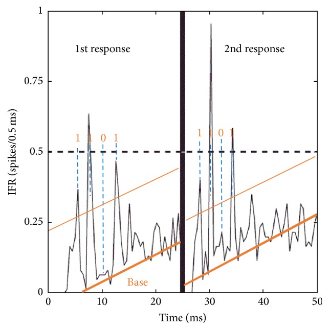
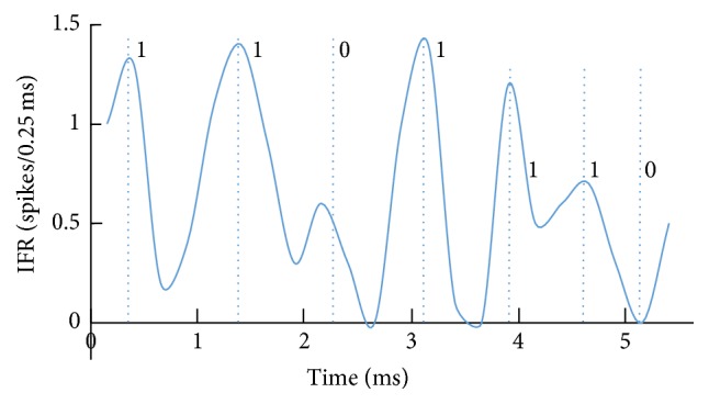
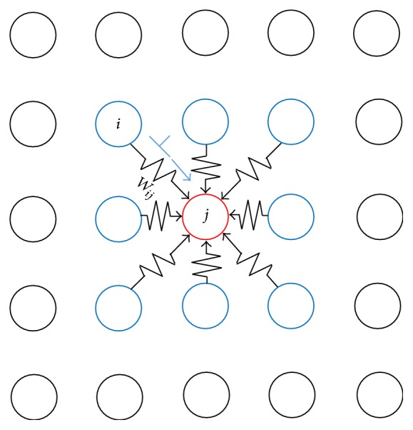
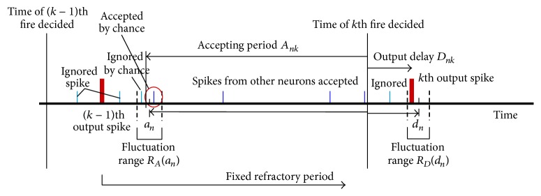
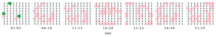
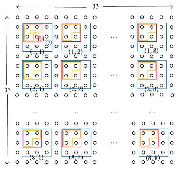
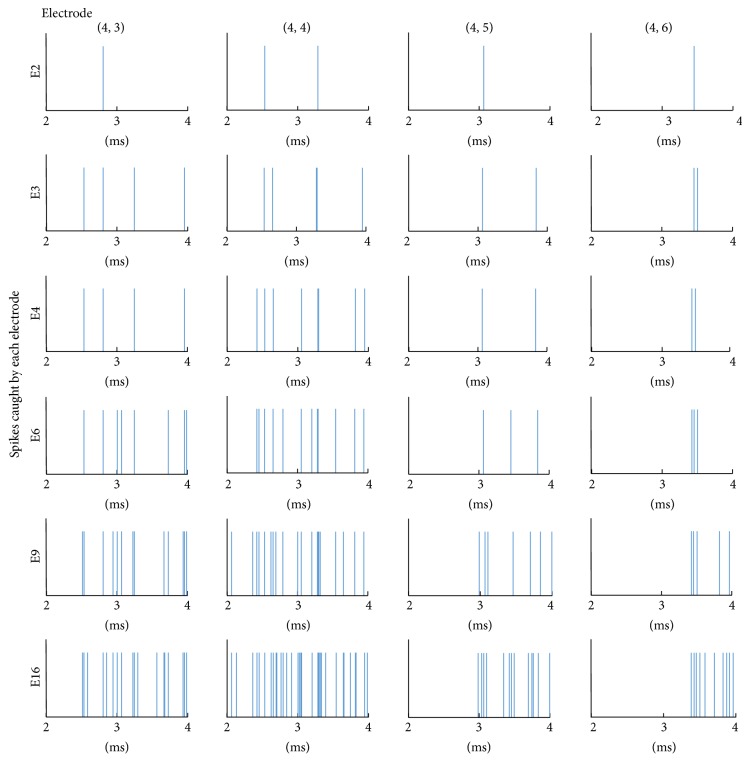
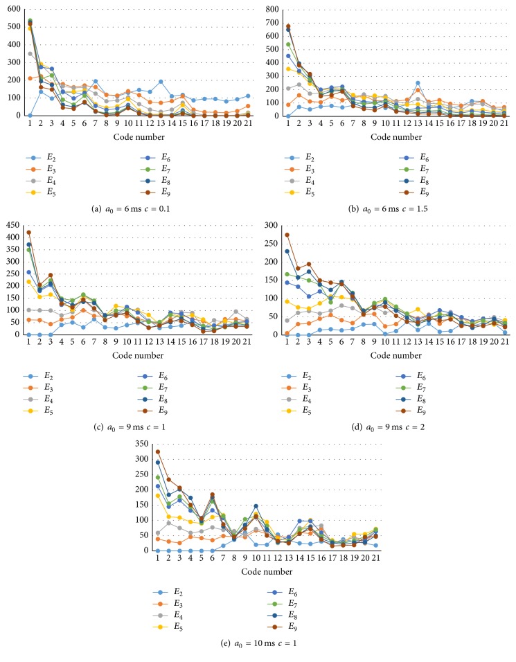
It has been shown that, in cultured neuronal networks on a multielectrode, pseudorandom-like sequences (codes) are detected, and they flow with some spatial decay constant. Each cultured neuronal network is characterized by a specific spectrum curve. That is, we may consider the spectrum curve as a "signature" of its associated neuronal network that is dependent on the characteristics of neurons and network configuration, including the weight distribution. In the present study, we used an integrate-and-fire model of neurons with intrinsic and instantaneous fluctuations of characteristics for performing a simulation of a code spectrum from multielectrodes on a 2D mesh neural network. We showed that it is possible to estimate the characteristics of neurons such as the distribution of number of neurons around each electrode and their refractory periods. Although this process is a reverse problem and theoretically the solutions are not sufficiently guaranteed, the parameters seem to be consistent with those of neurons. That is, the proposed neural network model may adequately reflect the behavior of a cultured neuronal network. Furthermore, such prospect is discussed that code analysis will provide a base of communication within a neural network that will also create a base of natural intelligence.

Figure 1

First and second responses “1101” in the instantaneous firing rate (IFR) of cultured neuronal tissue after two electrical stimulations as shown in [15] with additional interpretation (courtesy of Baljon et al.; reproduction permission provided by APS).

Figure 2

Instantaneous firing rate (poststimulus time histogram) where the sequence “1101” was observed. Since the timing becomes dispersed within trials, the peak positions and shapes gradually changed as time elapsed. Particularly, there was a tendency of risings and peaks to become faster than the regular timing, which is led by the fastest spike among the dispersed spikes as well as the slowest spike to be cancelled by the succeeding fastest negative spike (effectively supposed; pulling down the tail of peak), and lowering the peak height [16, 17].

Figure 3

Inputs to neuron j in a 2D mesh neural network. Each neuron j (red) receives input spikes from eight neighboring neurons (blue) such as i through connection weights w _ij ∈ [−1,1]. Neuron j integrates such weighted spikes during its accepting period and outputs a spike after a delay time if the integrated value exceeds zero.

Figure 4

Integrate-and-fire model without leakage but with fluctuation in the parameters of neuron n. Each neuron has an inherent accepting period a _n and output delay time d _n. These parameters vary with time within certain ranges R _A(a _n) and R _D(d _n), respectively. Neuron n integrates weighted input spikes during the accepting period A _nk for the kth firing, and after the refractory period ends, it decides whether the integrated value exceeds zero for firing at every time point. If so, it outputs the kth output spike with delay time D _nk. That is, A _nk ∈ R _A(a _n), and likewise, D _nk ∈ R _D(d _n).

Figure 5

Spike waves generated on a 2D mesh neural network. Green spots indicate stimulation point. “0.1–0.5 ms” means an accumulation result of firing at 0.1 ms, 0.2 ms,…, 0.5 ms. This suggests that the codes are a part of these “spike waves.”

Figure 6

Arrangement of 8 × 8 multi-electrodes [(1,1), (1,2),…, (8,8)] on a simulated 33 × 33 2D mesh neural network. Each electrode acquires spikes of two to nine neurons. For example, “E9” showing 3 × 3 block of neurons (○) indicated with (1,1) shows that electrode (1,1) collects spikes from nine neurons. In addition, “E3” and “E4” are likewise; “E2” and “E5”–“E8”are not shown. Spectrum, cross-correlation, or probability distribution data obtained from electrode Em is expressed as “E _m” in the text. Connections between eight neighboring neurons are randomly generated with given stochastic characteristics.

Figure 7

An example of simulated spike trains caught by Em during 2.0–4.0 ms after stimulation with a ₀ = 8.0 ms and c = 2.5. Initial stimulations were given to around electrodes (1,1) at 0.1 ms and (1,5) at 0.5 ms.

Figure 8

Code spectrum components E _m for several parameters of accepting period a ₀ and positive and negative weight balance c. The horizontal line represents code numbers (1,2,…, 21) whose number of “1”s in the code is 3. That is, code 1 = “111,” code 2 = “1011,” code 3 = “1101,” code 4 = “10011,” code 5 = “10101,” … code 21 = “11000001” [22]. The vertical line represents the total number of codes detected during the first 200 ms after stimulation (2000 time bins of 0.1 ms/bin) and from 63 electrodes.

Figure 9

Code spectra. The blue curve shows the average of trials of an experimental number of codes detected from 63 electrodes in spike trains during 200 ms after stimulation expressed with 2000 time bins of 0.1 ms. The bit width of the code is 0.6–2.0 ms (6–20 bins). Codes are detected with 1% time accuracy, although practically several % because of the 0.1 ms bit width. This curve can be considered as the “signature” of spike trains. The orange curve is the best fit to code spectrum using a simulation spectrum.

Figure 10

Expanded spectrum components up to E ₁₆. (a) Code spectrum components E ₂–E ₉ for a ₀ = 7 ms and c = 2. (b) Expansion to E ₉–E ₁₆ of (a). (c) Code spectrum components E ₂–E ₉ for a ₀ = 8 ms and c = 2.5. (d) Expansion to E ₉–E ₁₆ of (c).

Figure 11

Maximum cross-correlation Φ_N(C) of a trial among eight (8N) and 20 (20N) neighbors with a time frame difference of 0.5 ms for 14 major codes C.

Figure 12

Time-shift diagram of 10.2 Hz MEG, for a number counting task [23, 24]. Red arrow < 5 ms < green < 10 ms < blue. We can see that red arrow with lag time < 5 ms runs within each hemisphere, and blue > 10 ms across the callosum.

Figure 13

Illustration of the communication within the neural network based on spatiotemporal pattern recognition. Each neuron can perform the roles of transmitting, receiving, and simply as a transmission media.

References

-
- Kliper O., Horn D., Quenet B., Dror G. Analysis of spatiotemporal patterns in a model of olfaction. Neurocomputing. 2004;58–60:1027–1032. doi: 10.1016/j.neucom.2004.01.162. - DOI
- Mohemmed A., Schliebs S., Matsuda S., Kasabov N. Training spiking neural networks to associate spatio-temporal input-output spike patterns. Neurocomputing. 2013;107:3–10. doi: 10.1016/j.neucom.2012.08.034. - DOI
MeSH terms
LinkOut - more resources
Full Text Sources
Other Literature Sources