Mining 3D genome structure populations identifies major factors governing the stability of regulatory communities

Abstract

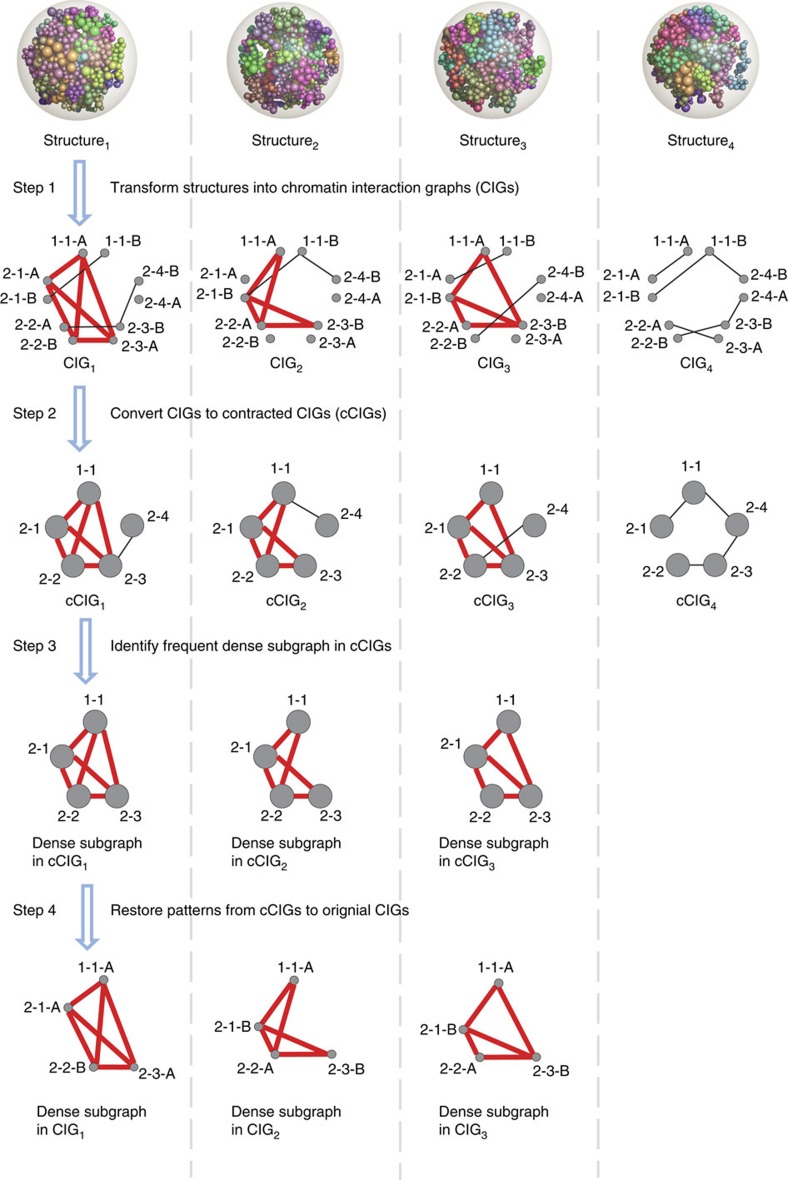
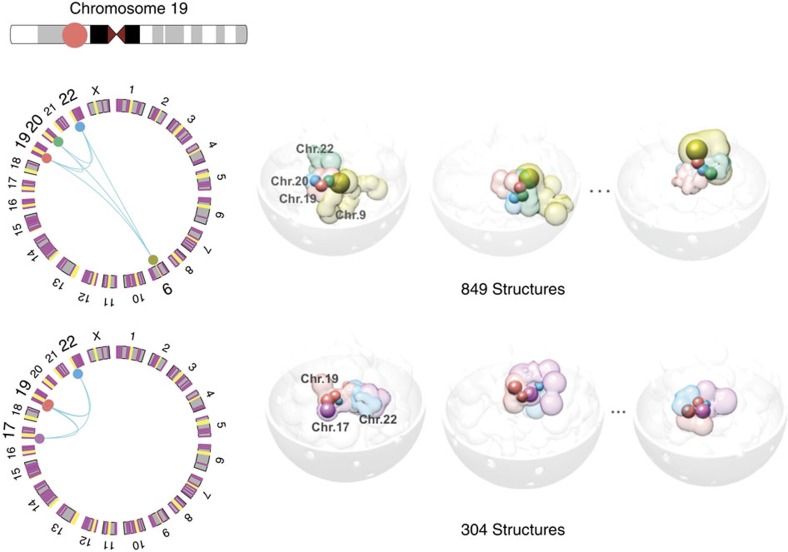
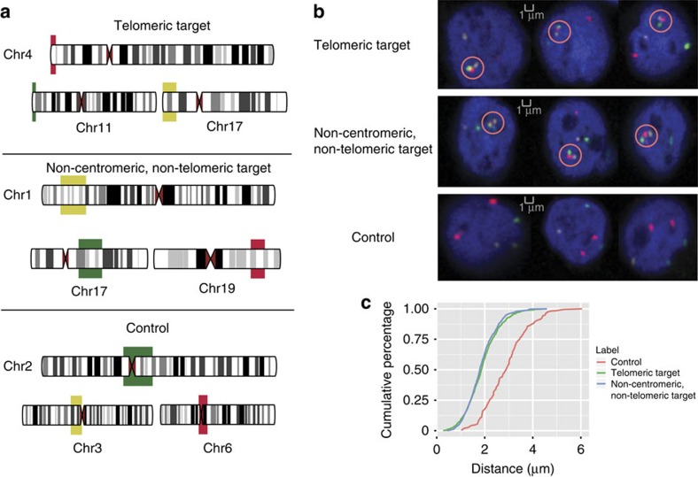
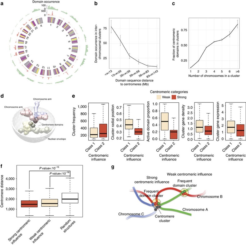
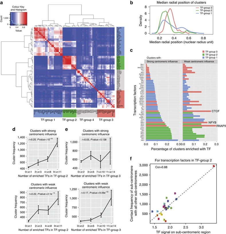
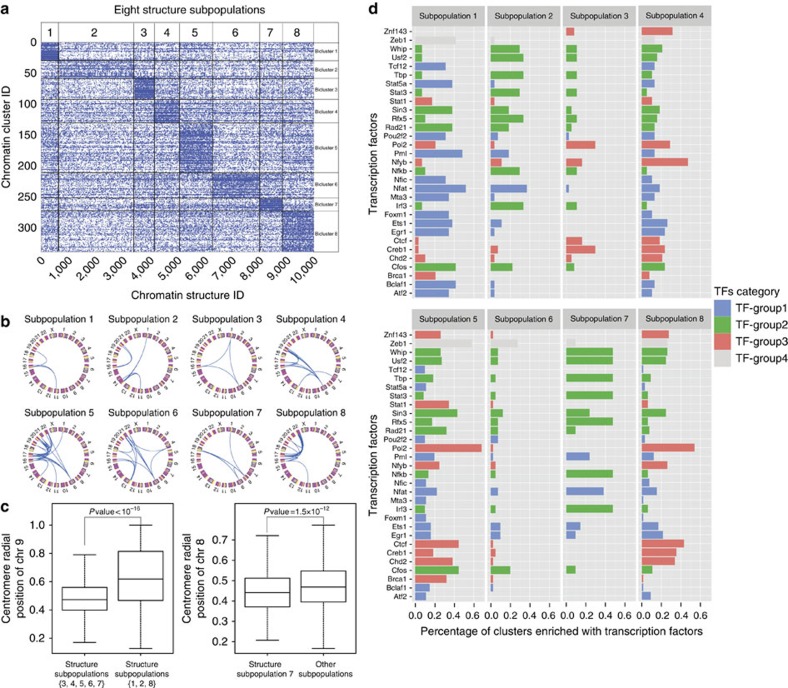
Three-dimensional (3D) genome structures vary from cell to cell even in an isogenic sample. Unlike protein structures, genome structures are highly plastic, posing a significant challenge for structure-function mapping. Here we report an approach to comprehensively identify 3D chromatin clusters that each occurs frequently across a population of genome structures, either deconvoluted from ensemble-averaged Hi-C data or from a collection of single-cell Hi-C data. Applying our method to a population of genome structures (at the macrodomain resolution) of lymphoblastoid cells, we identify an atlas of stable inter-chromosomal chromatin clusters. A large number of these clusters are enriched in binding of specific regulatory factors and are therefore defined as 'Regulatory Communities.' We reveal two major factors, centromere clustering and transcription factor binding, which significantly stabilize such communities. Finally, we show that the regulatory communities differ substantially from cell to cell, indicating that expression variability could be impacted by genome structures.

Figure 1. The overall procedure to discover frequent dense clusters.

Each 3D genome structure is transformed into a CIG where a node represents a domain and an edge represents a contact between two domains. In this example, 4 CIGs with 10 nodes are built. Each node is labelled by the triplet L1–L2–L3, where L1 indicates the chromosome index, L2 indicates the domain index among all domains in its chromosome and L3 (a letter A or B) indicates which copy of the chromosome the domain comes from. For example, nodes 2-3-A and 2-3-B indicate ‘twin' nodes are from the 3rd domain of chromosome 2, in its two homologous copies. Step 1: Each genome structure is transformed into a CIG. Step 2: in each CIG, we merge any two ‘twin' nodes that represent homologous domains. This step yields a collection of four contracted graphs without isomorphism (termed cCIG, where each node is a merged domain, labelled by L1 and L2). Step 3: We identify the dense subgraphs that frequently occur across many networks using a tensor-based computational method. Step 4: We restore each frequent dense subgraph to its un-contracted form in the original CIGs, and after mining on these subgraphs with ‘coupled isomorphism' we identify the final set of frequent dense subgraphs.

Figure 2. Functional plasticity of chromatin domain.

An active domain in chromosome 19 can participate in two different clusters that are enriched with binding of the same transcription factors, including RNAPII, CTCF, NFYB and CREB1.

Figure 3. 3D FISH experiments to validate the co-localization of domains within two inter-chromosomal clusters.

(a) Layout of the 3D FISH experiments where the chromosomal locations of the clustered (targeted) regions and the control regions are shown. Telomeric targets were from p-arm telomeric regions of chromosome 4, 11 and 17. Non-centromeric, non-telomeric targets were from chromosomes 1, 17 and 19. Control regions were from sub-centromeric regions of chromosomes 2, 3 and 6. (b) Three example images of 3D FISH results in interphase nuclei are shown for telomeric target, non-centromeric, non-telomeric target and control regions, respectively. We used green, red, and yellow to label genomic locations of target and control regions. The chromosomal DNA was counterstained in blue with DAPI. Note that for the best view, the targeted region was the overlaid image of four channels (blue, green, yellow and red) from one of the exactly same Z-section, whereas the image of the control cell was the Z-projection of all z-sections from four channels. (c) Cumulative percentage of the average distances of the clustered targeted regions or the control regions were calculated from all the cells analysed (943 cells in telomeric targets, 982 cells in non-centromeric, non-telomeric targets and 595 cells in control regions). For two homologous regions of each chromosome, only one with the shortest distance from other chromosomes was counted and subject to analysis. In each cell, the distance (x-axis) was calculated as the average distance among three FISH probes.

Figure 4. Centromeric influence on spatial clusters.

(a) Domain occurrence in frequent spatial clusters. The full set of chromosomes is represented as the circular plot, where centromeric domains are coloured as yellow, active domains are coloured as red and inactive/other domains are coloured as grey. (b) A plot measuring the correlation between linear centromeric distance and domain occurrence in inter-chromosomal clusters. Data are shown as mean±s.d. of the mean. The number of domains in each group is 73, 72, 72, 73, 72 and 72. (c) A plot showing the correlation between the number of chromosomes in a cluster and the fraction of centromeric domains in the cluster. Data are shown as mean±s.d. of the mean. The number of clusters in each group is 749, 834, 1059, 972, 192, 36 and 14. (d) Illustration of centromere–centromere clustering. (e) Box plots comparing the characteristics of inter-chromosomal clusters with strong and weak centromeric influence, in terms of frequency, radial position, active domain proportion, gene density (the number of genes per 100 kb) and gene expression. (f) Box plots comparing centromere distance between three groups: clusters with strong centromeric influence, clusters with weak centromeric influence and clusters with weak centromeric influence that in random structures. (g) Illustration of inter-chromosomal clusters with strong and weak centromeric influence.

Figure 5. Transcription factors stabilization effects on spatial clusters.

(a) About 65 TFs are classified into 4 groups based on their enrichment profiles across all inter-chromosomal clusters. (b) Radial position distributions of inter-chromosomal clusters exclusively enriched with individual TF-group. (c) Comparison of inter-chromosomal clusters with strong versus weak centromeric influence, in terms of the percentages of clusters enriched in TFs from different TF groups. (d) Correlation plot between cluster frequency and the number of enriched TFs in Group 2 with strong/weak centromeric influence. Data are shown as mean±s.d. of the mean. For clusters with strong centromeric influence, the number of clusters in each group is 339, 60, 230 and 220. For clusters with weak centromeric influence, the number of clusters in each group is 257, 69, 89 and 94. (e) Correlation plot between cluster frequency and the number of enriched TFs in Group 3 with strong/weak centromeric influence. Data are shown as mean±s.d. of the mean. For clusters with strong centromeric influence, the number of clusters in each group is 1,609; 207; 47 and 18. For clusters with weak centromeric influence, the number of clusters in each group is 958, 137, 94 and 37. (f) Correlation plot between the Group 2 TF signals on sub-centromeric regions and the subcentromere–subcentromere contact frequencies.

Figure 6. Genome structure subpopulation analysis.

(a) 10,000 structures are partitioned into 8 non-overlapping subpopulations. (b) Each structure subpopulation has a distinct pattern of inter-chromosomal contacts, which display the top 20% high-frequency domain pairs. (c) Compare the radial position of specific chromosomes in different structure subpopulations. (d) The eight structure subpopulations have different top-enriched TFs.

References

1. Lieberman-Aiden E. et al.. Comprehensive mapping of long-range interactions reveals folding principles of the human genome. Science 326, 289–293 (2009). - PMC - PubMed
1. Duan Z. et al.. A three-dimensional model of the yeast genome. Nature 465, 363–367 (2010). - PMC - PubMed
1. Kalhor R., Tjong H., Jayathilaka N., Alber F. & Chen L. Genome architectures revealed by tethered chromosome conformation capture and population-based modelling. Nat. Biotechnol. 30, 90–98 (2012). - PMC - PubMed
1. Rao S. S. et al.. A 3D map of the human genome at kilobase resolution reveals principles of chromatin looping. Cell 159, 1665–1680 (2014). - PMC - PubMed
1. Fullwood M. J. et al.. An oestrogen-receptor-alpha-bound human chromatin interactome. Nature 462, 58–64 (2009). - PMC - PubMed
Publication types
LinkOut - more resources