Bayesian inference with Stan: A tutorial on adding custom distributions

Abstract

When evaluating cognitive models based on fits to observed data (or, really, any model that has free parameters), parameter estimation is critically important. Traditional techniques like hill climbing by minimizing or maximizing a fit statistic often result in point estimates. Bayesian approaches instead estimate parameters as posterior probability distributions, and thus naturally account for the uncertainty associated with parameter estimation; Bayesian approaches also offer powerful and principled methods for model comparison. Although software applications such as WinBUGS (Lunn, Thomas, Best, & Spiegelhalter, Statistics and Computing, 10, 325-337, 2000) and JAGS (Plummer, 2003) provide "turnkey"-style packages for Bayesian inference, they can be inefficient when dealing with models whose parameters are correlated, which is often the case for cognitive models, and they can impose significant technical barriers to adding custom distributions, which is often necessary when implementing cognitive models within a Bayesian framework. A recently developed software package called Stan (Stan Development Team, 2015) can solve both problems, as well as provide a turnkey solution to Bayesian inference. We present a tutorial on how to use Stan and how to add custom distributions to it, with an example using the linear ballistic accumulator model (Brown & Heathcote, Cognitive Psychology, 57, 153-178. doi: 10.1016/j.cogpsych.2007.12.002 , 2008).

Keywords: Bayesian inference; Linear ballistic accumulator; Probabilistic programming; Stan.

Probability density function of the LBA, snipped from Box 4 in the main text.

Cumulative distribution function of the LBA, continued from Box A1

LBA random number generator (RNG). The model assumes that on every trial at least one of the drift rates is positive. Code is continued from Box A2.

Fig. 1. Autocorrelation function of the rate parameter

Fig. 2. Samples from each chain as a function of iteration generated by Stan (left) and Metropolis–Hastings (right)

Fig. 3. A posterior predictive check (left), where the solid line represents the predictions and the histogram bars represent the data, and the posterior distribution of λ (right)

Fig. 4. Actual parameter values plotted as a function of the recovered parameter values for Stan (left) and Metropolis– Hastings (right)

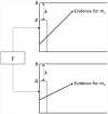
Fig. 5. Graphical depiction of the linear ballistic accumulator (LBA) model (Brown & Heathcote, 2008)

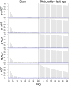
Fig. 6. Autocorrelation function (ACF) of each parameter, plotted as a function of lag, for Stan (left) and Metropolis–Hastings (right)

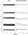
Fig. 7. Samples of each parameter for each iteration of each chain for Stan (left) and Metropolis–Hastings (right)

Fig. 8. Actual parameter values, plotted as a function of the parameters recovered by Stan (left) and Metropolis–Hastings (right)

Fig. 9

The lower left of the grid shows the joint posterior probability distributions for each pair of key parameters in the LBA model fitted to a simulated set of data. Each point in each panel represents a posterior sample from the joint posterior probability distribution of a particular parameter pair for the LBA model. For example, the bottom left corner panel shows the joint posterior probability distribution between τ and v₁. The upper right of the grid gives the correlation between each parameter pair. For example, the upper right corner shows the correlation between τ and v₁ to be −.45

Fig. 10

Group-level parameter estimates of the hierarchical LBA model for simulated data. For the panels plotting v₁ and v₂, solid lines indicate Condition 1, dotted lines indicate Condition 2, and dashed lines indicate Condition 3

Fig. 11. Hierarchical model parameter estimates (solid lines) versus nonhierarchical parameter estimates (dashed lines) for a single subject in a single condition

References

1. Brooks S, Gelman A, Jones GL, Meng XL. Handbook of Markov chain Monte Carlo. Boca Raton, FL: Chapman & Hall/CRC; 2011.
1. Brown SD, Heathcote A. The simplest complete model of choice reaction time: Linear ballistic accumulation. Cognitive Psychology. 2008;57:153–178. doi: 10.1016/j.cogpsych.2007.12.002. - DOI - PubMed
1. Donkin C, Brown SD, Heathcote A. The overconstraint of response time models: Rethinking the scaling problem. Psychonomic Bulletin & Review. 2009;16:1129–1135. doi: 10.3758/PBR.16.6.1129. - DOI - PubMed
1. Duane S, Kennedy AD, Pendleton BJ, Roweth D. Hybrid Monte Carlo. Physics Letters B. 1987;195:216–222.
1. Gelman A, Carlin JB, Stern HS, Dunson DB, Vehtari A, Rubin DB. Bayesian data analysis. 3rd. Boca Raton, FL: Chapman & Hall/CRC; 2013.
LinkOut - more resources