Three-dimensional spatiotemporal focusing of holographic patterns

Abstract

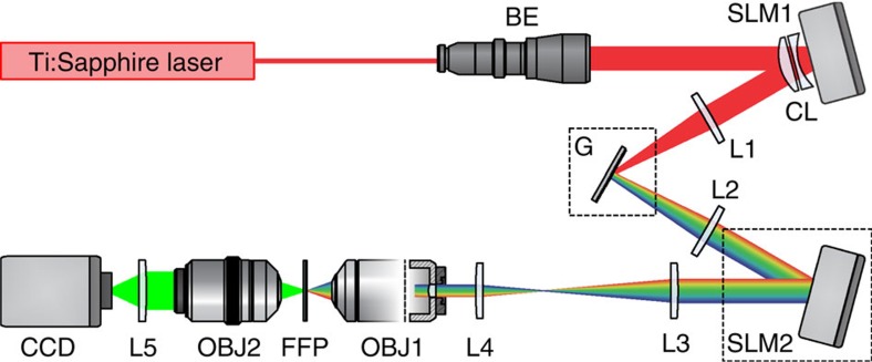
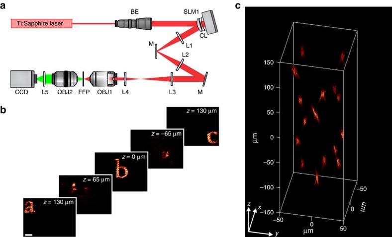
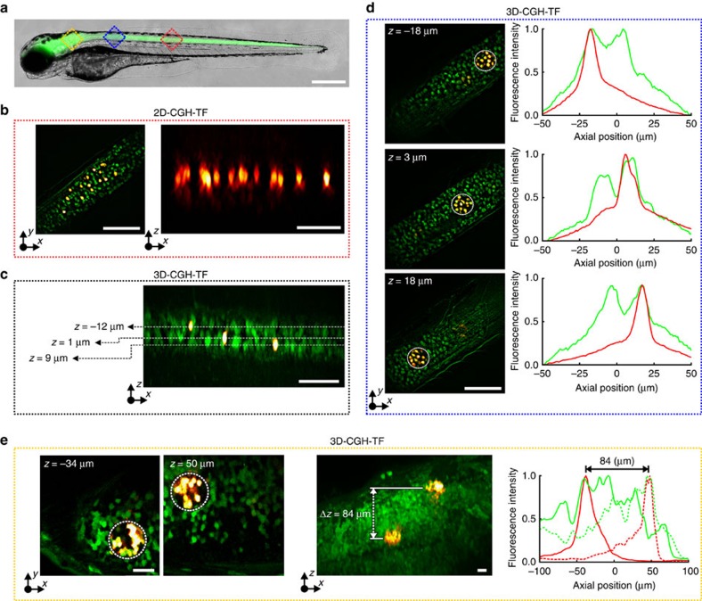
Two-photon excitation with temporally focused pulses can be combined with phase-modulation approaches, such as computer-generated holography and generalized phase contrast, to efficiently distribute light into two-dimensional, axially confined, user-defined shapes. Adding lens-phase modulations to 2D-phase holograms enables remote axial pattern displacement as well as simultaneous pattern generation in multiple distinct planes. However, the axial confinement linearly degrades with lateral shape area in previous reports where axially shifted holographic shapes were not temporally focused. Here we report an optical system using two spatial light modulators to independently control transverse- and axial-target light distribution. This approach enables simultaneous axial translation of single or multiple spatiotemporally focused patterns across the sample volume while achieving the axial confinement of temporal focusing. We use the system's capability to photoconvert tens of Kaede-expressing neurons with single-cell resolution in live zebrafish larvae.

Figure 1. Experimental set-up for 3D-CGH-TF.

The output beam of a Ti:Sapphire laser is magnified using a beam expander (BE) and projected on a first SLM (SLM1). SLM1 modulates the beam's phase so that light forms a user-defined intensity pattern on the diffraction grating (G) after passing through lens L1. The first diffraction order is collimated by the lens L2 and directed on a second SLM (SLM2). SLM2 imprints a lens-phase modulation that enables precise axial positioning of the spatiotemporal focal plane. The laser beam is then relayed and scaled by lenses L3 and L4 to the excitation objective (OBJ1) pupil size. OBJ1 is mounted on a piezo positioner so that it focuses and axially scans the excitation beam across a thin fluorescent layer. A second objective (OBJ2), always focused on the fluorescent layer, collects emitted fluorescence and forms an image on a CCD camera. Two cross-oriented cylindrical lenses (CL), with focal lengths of equal power and opposite sign, are used to suppress the zero-order spot of the first SLM.

Figure 2. Axial displacement of spatiotemporally focused patterns.

(a) Axial displacement of a 20-μm-diameter temporally focused holographic spot. Top, orthogonal maximum fluorescence intensity projection of the spot, for axial displacements of ±50 and±100 μm from the focal plane (0 μm). Bottom, corresponding x–y fluorescence intensity cross-sections. Scale bar, 20 μm. The colour bar refers to normalized intensity. (b) Axial profile of the integrated fluorescence intensity of the 20-μm-diameter holographic spot for different axial displacements. (c) Axial confinement (FWHM) of the profiles shown in b (CGH-TF; red data) compared with the axial confinement of a 20-μm-diameter holographic spot without TF (CGH; blue data). Data were fitted with a parabolic function (dashed lines) in both cases. White area in b,c represents the field of excitation (FOE_z).

Figure 3. Multiplane spatiotemporally focused pattern generation.

(a) Top, tiled phase profiles addressed to SLM1 for encoding the words ‘neuro' (plane A) and ‘photonics' (plane B). Bottom, Fresnel lens-phase profiles addressed to SLM2 to axially displace each holographic pattern generated by SLM1 on separated planes at +20 μm (plane A) and −20 μm (plane B). (b) Left, x–y 2P fluorescence intensity cross-sections at planes A and B generated by the holograms in a. Right, orthogonal maximum 2P intensity projection along x (top) and y (bottom). (c) Orthogonal fluorescence intensity projection of spatiotemporally focused patterns created by projecting 20-μm-diameter holographic spots in one, two, three and four planes at positions laterally shifted and in four planes at positions axially aligned (from left to right). Scale bars, 20 μm. (d) Axial confinement (FWHM) of a 20-μm-diameter holographic spot for different hologram widths, tested in both directions, Δ_x (blue data) and Δ_y (red data) parallel and perpendicular to grating's dispersion, respectively. (e) x–y 2P fluorescence intensity cross-sections of a 20-μm-diameter holographic spot generated with different hologram widths Δ_y. (f) Autocorrelation width at the sample plane of a 20-μm-diameter holographic spot as a function of the hologram width along the x- (blue data; σ_x) and y directions (red data; σ_y). (g) Axial profile of the integrated fluorescence intensity of the holographic spots shown on c. Colour bars refer to normalized intensity.

Figure 4. 3D-CGH.

(a) Schematic of the optical set-up for 3D-CGH. In this case the diffraction grating G and SLM2 were replaced by mirrors. (b) 2P fluorescence images of 3D-CGH patterns, depicting the letters ‘a', ‘b' and ‘c' at three different axial positions, z=130 μm, 0 and −130 μm, respectively. The phase profile used to project these patterns was calculated using a multiplane GS algorithm (Supplementary Fig. 9). Weighting of the input patterns according to their lateral and axial position (Supplementary Fig. 3) enabled diffraction efficiency correction and generated equal-intensity light patterns. (c) Volumetric reconstruction of three-dimensional distribution of 5-μm-diameter holographic spots (see also Supplementary Movie 1).

Figure 5. 3D simultaneous 2P photoconversion of Kaede in vivo.

(a) Merged brightfield and widefield fluorescence images of a double transgenic Tg(HuC:gal4; UAS:kaede) zebrafish larvae. Red and blue squares represent the approximate areas where we performed photoconversion. Scale bar, 400 μm. (b) Left, overlaid green and red HiLo fluorescence images before and after photoconversion, respectively. Right, orthogonal maximum red fluorescence intensity projection showing 14 photoconverted neurons on a single axial plane (illumination density 0.4 mW μm⁻², 200 pulses of 50 ms). Scale bars, 60 μm. (c) Orthogonal maximum fluorescence intensity projection of overlaid HiLo pre- and post-photoconversion images (green and red fluorescence, respectively). Three single cells were photoconverted on separated axial planes (4.0 mW μm⁻², one pulse of 200 ms). Scale bar, 60 μm. (d) Simultaneous 3D photoconversion of neural ensembles in the spinal cord. Left, overlaid HiLo pre- and post-photoconversion fluorescence images, where three 35-μm-diameter holographic spots projected at z=−18 μm, 3 and 18 μm were used for photoconversion (0.03 mW μm⁻², 2,000 pulses of 50 ms). Right, axial distributions of green pre- and red post-photoconversion integrated fluorescence intensity over z for the spots projected at the three different planes. Scale bars, 60 μm. (e) Simultaneous 3D photoconversion of neural ensembles in the zebrafish brain. Left, overlaid 2P-excited green- and red post-photoconversion fluorescence images, where two 35-μm-diameter holographic spots projected at z=−38 μm and 50 μm were used for photoconversion (0.11 mW μm⁻², 9,000 pulses of 50 ms). Scale bar, 20 μm. Middle, Orthogonal maximum 2P-excited fluorescence intensity projection of overlaid green and red-post-photoconversion images. Scale bar, 20 μm. Right, axial distributions of green pre- and red post-photoconversion integrated 2P fluorescence intensity over z for the spot at z=−38 μm (solid lines) and the one at z=50 μm (dotted lines). z-values in all cases are given as distances from the focal plane of the objective, which for the spinal cord experiments was at ∼60 μm and for the brain at ∼90 μm from the fish surface (where green fluorescence was starting). Positive z-values are closer to the surface. λ_phot=800 nm.

References

1. Denk W., Strickler J. H. & Webb W. W. Two-photon laser scanning fluorescence microscopy. Science 248, 73–76 (1990). - PubMed
1. Salomé R. et al. Ultrafast random-access scanning in two-photon microscopy using acousto-optic deflectors. J. Neurosci. Methods 154, 161–174 (2006). - PubMed
1. Reddy G. D., Kelleher K., Fink R. & Saggau P. Three-dimensional random access multiphoton microscopy for functional imaging of neuronal activity. Nat. Neurosci. 11, 713–720 (2008). - PMC - PubMed
1. Grewe B. F., Langer D., Kasper H., Kampa B. M. & Helmchen F. High-speed in vivo calcium imaging reveals neuronal network activity with near-millisecond precision. Nat. Methods 7, 399–405 (2010). - PubMed
1. Nguyen Q. T., Callamaras N., Hsieh C. & Parker I. Construction of a two-photon microscope for video-rate Ca2+ imaging. Cell Calcium 30, 383–393 (2001). - PubMed
Publication types
MeSH terms
LinkOut - more resources