Defining and quantifying the resilience of responses to disturbance: a conceptual and modelling approach from soil science

Abstract

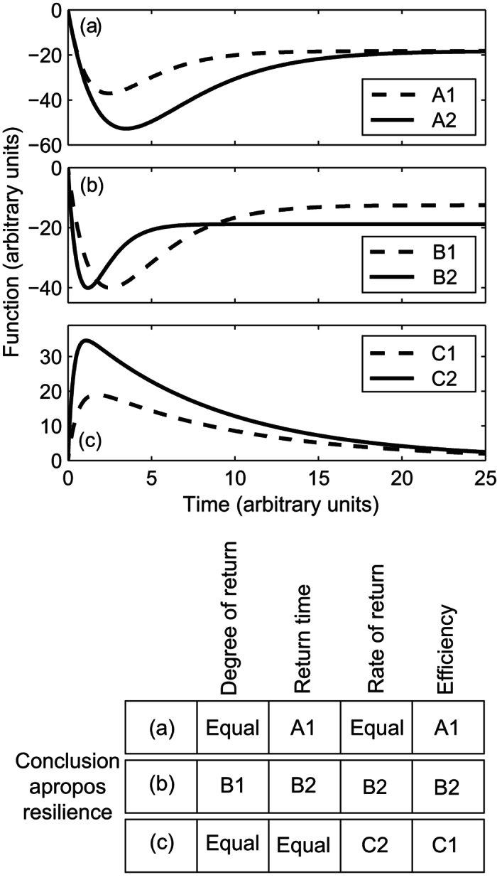
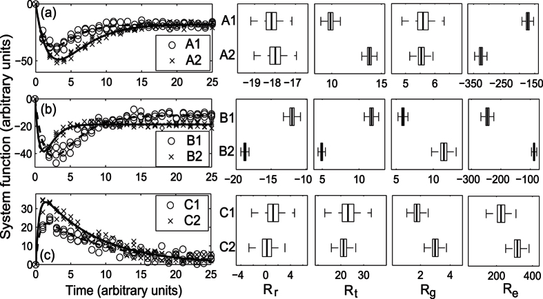
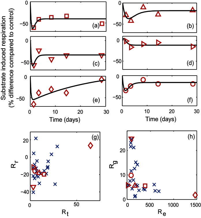
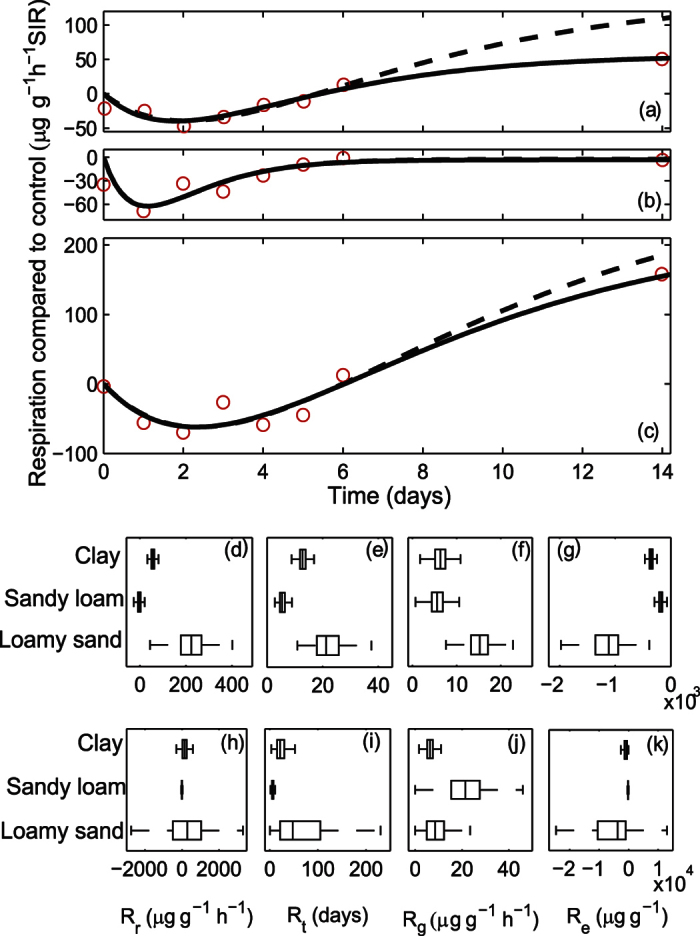
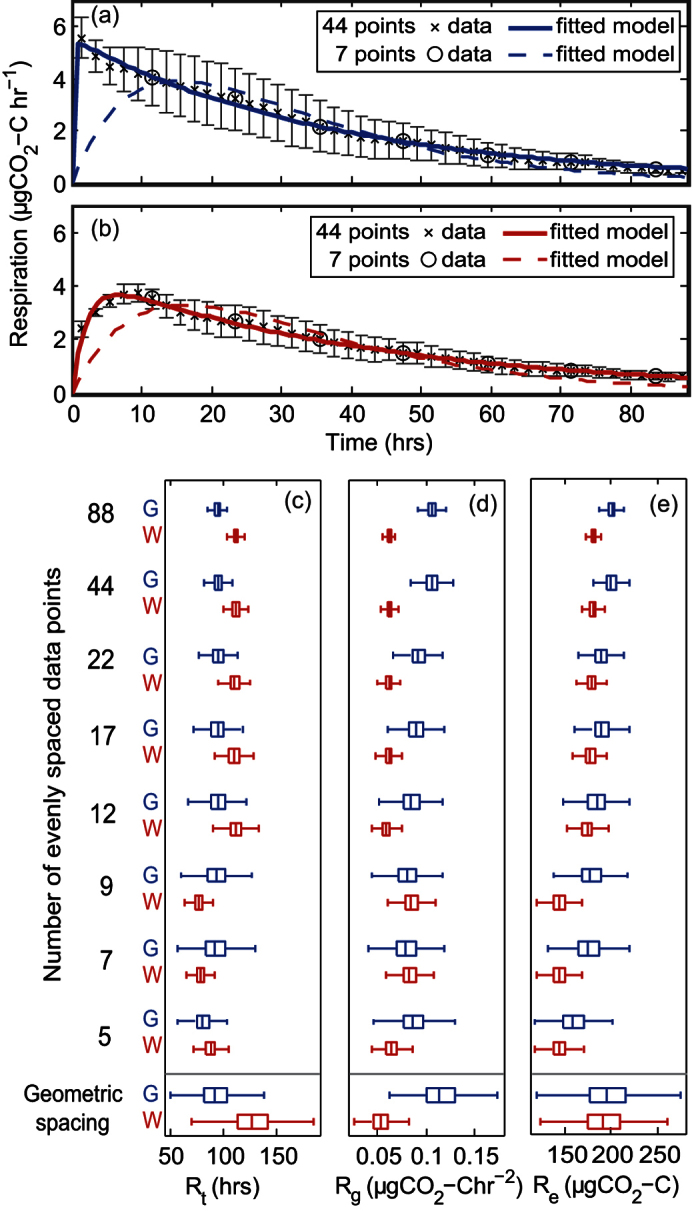
There are several conceptual definitions of resilience pertaining to environmental systems and, even if resilience is clearly defined in a particular context, it is challenging to quantify. We identify four characteristics of the response of a system function to disturbance that relate to "resilience": (1) degree of return of the function to a reference level; (2) time taken to reach a new quasi-stable state; (3) rate (i.e. gradient) at which the function reaches the new state; (4) cumulative magnitude of the function (i.e. area under the curve) before a new state is reached. We develop metrics to quantify these characteristics based on an analogy with a mechanical spring and damper system. Using the example of the response of a soil function (respiration) to disturbance, we demonstrate that these metrics effectively discriminate key features of the dynamic response. Although any one of these characteristics could define resilience, each may lead to different insights and conclusions. The salient properties of a resilient response must thus be identified for different contexts. Because the temporal resolution of data affects the accurate determination of these metrics, we recommend that at least twelve measurements are made over the temporal range for which the response is expected.

Figure 1

Comparisons of three, hypothetical pairs of responses (a–c) to a disturbance and (table inset) the conclusions that can be drawn to identify which of each pair is more resilient when comparing the four resilience characteristics identified in Table 1.

Figure 2

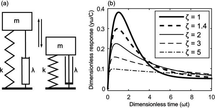
(a) Diagram of the mechanical spring damper system, with mass m, spring constant k and damping constant λ, used as an analogy to develop a model of soil function perturbation after a disturbance. (b) The dimensionless response of this spring damper system for different damping factors (), plotted for a new equilibrium position at . See Supplementary Methods for derivation of formulae.

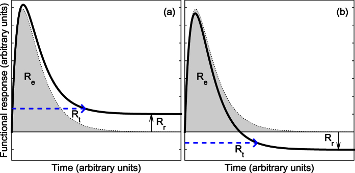
Figure 3. Diagrams to show how the resilience characteristics for degree of return (R_r), return time (R_t), and efficiency (R_e) are quantified from the modelled response curve.

R_g is quantified as the average magnitude of the gradient of the curve between 0 and R_t.

Figure 4

Synthetic data and simulated, fitted responses based on the three pairs of responses shown in Fig. 1 (a–c) along with values of degree of return (R_r), return time (R_t), rate of return (R_g) and efficiency (R_e) estimated from these fitted responses. Boxplots show the median (central mark), interquartile range (box) and range (whiskers) with outliers excluded.

Figure 5

Six indicative examples (a–f) of the response of SIR after exposure to heat stress showing the derived resilience metrics (g,h) (R_r, R_t, R_g and R_e, Table 1) for the 24 soil samples in which the model identified the degree of return. Symbols in plots (g,h) correspond to those in the responses plots (a–f), metrics for the responses of other soils are shown as crosses. Confidence intervals for these metrics are large (due to the small number of data points) and are not shown. Different soils are identified as more resilient depending on which characteristic is used to rank the responses. For example, the response in plot (c) is identified as the most resilient using the rate of return metric (R_g) because the gradient during the response period is large. However, it is one of the least resilient responses in terms of the degree of return (R_r) as it returns to a level which is very different to that of the control (i.e. far from zero). The response in plot (e) is identified as the least resilient using all the metrics except R_r as it eventually returns to a level similar to that of the control.

Figure 6

Change in substrate induced respiration of (a) clay, (b) sandy loam and (c) loamy sand soil samples after the addition of 1000 mg triclosan kg⁻¹ dry mass showing data (circles) and the modelled response fitted either with (solid lines) or without (dashed lines) the last data point. Note that the two modelled responses are almost identical in the sandy loam. Measurements are the difference in SIR (glucose substrate) between a perturbed and a control sample, with each measurement made destructively. The resilience characteristics (Table 1) identified using the model fitted to all the data (d–g) and the model fitted without the last data point (h–k). Boxplots show the median (central mark), interquartile range (box) and range (whiskers) with outliers excluded.

Figure 7

Respiration responses observed after a drying and rewetting disturbance in (a) grassland, sandy loam soil and (b) woodland, clay loam soil and the corresponding modelled results when fitted to two subsets of the full time series. Error bars indicate ± standard deviation of the data. The estimated (c) return time (R_t), (d) rate of return (R_g), and (e) efficiency (R_e) characteristics for both soils (grassland–G, and woodland–W) are shown, each estimated using models fitted to subsets of the data with different numbers of data points evenly spaced throughout the measurement period and a geometric spacing of 7 measurements at 1, 2, 4, 8, 16, 32 and 64 hours. Boxplots show the median (central mark), interquartile range (box) and range (whiskers) with outliers excluded, this data is provided in Supplementary Dataset 1. The degree of return was fixed at zero during fitting, as the degree of return was small relative to the peak of the signal and the soils did not return to a stable respiration during the measurement period.

References

1. Desjardins E., Barker G., Lindo Z., Dieleman C. & Dussault A. C. Promoting Resilience. Q. Rev. Biol. 90, 147–65 (2015). - PubMed
1. Hodgson D., McDonald J. L. & Hosken D. J. What do you mean, ‘resilient’? Trends Ecol. Evol. 30, 503–6, ( 10.1016/j.tree.2015.06.010) (2015). - DOI - PubMed
1. Xu L., Marinova D. & Guo X. Resilience thinking: a renewed system approach for sustainability science. Sustain. Sci. 10, 123–38, ( 10.1007/s11625-014-0274-4) (2015). - DOI
1. Holling C. S. Resilience and stability of ecological systems. Annu. Rev. Ecol. Syst. 1–23, ( 10.1146/annurev.es.04.110173.000245) (1973). - DOI
1. Myers-Smith I. H., Trefry S. A. & Swarbrick V. J. Resilience: Easy to use but hard to define. Ideas Ecol. Evol. 5, ( 10.4033/iee.2012.5.11.c) (2012). - DOI
Publication types
LinkOut - more resources