. 2016 May;67(2):705-723.
doi: 10.1007/s10915-015-0099-z. Epub 2015 Sep 12.

Numerical Treatment of Stokes Solvent Flow and Solute-Solvent Interfacial Dynamics for Nonpolar Molecules

Affiliations

Numerical Treatment of Stokes Solvent Flow and Solute-Solvent Interfacial Dynamics for Nonpolar Molecules

Hui Sun et al. J Sci Comput. 2016 May.

Abstract

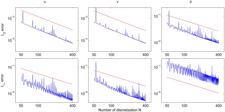
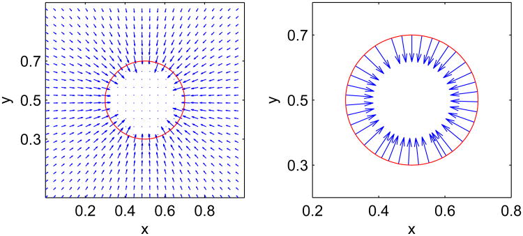
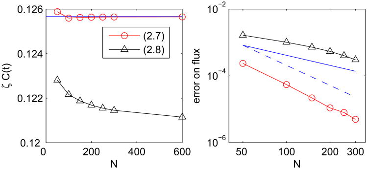
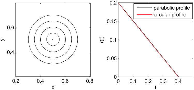
We design and implement numerical methods for the incompressible Stokes solvent flow and solute-solvent interface motion for nonpolar molecules in aqueous solvent. The balance of viscous force, surface tension, and van der Waals type dispersive force leads to a traction boundary condition on the solute-solvent interface. To allow the change of solute volume, we design special numerical boundary conditions on the boundary of a computational domain through a consistency condition. We use a finite difference ghost fluid scheme to discretize the Stokes equation with such boundary conditions. The method is tested to have a second-order accuracy. We combine this ghost fluid method with the level-set method to simulate the motion of the solute-solvent interface that is governed by the solvent fluid velocity. Numerical examples show that our method can predict accurately the blow up time for a test example of curvature flow and reproduce the polymodal (e.g., dry and wet) states of hydration of some simple model molecular systems.

Keywords: Nonpolar molecules; change of volume; ghost fluid method; interface motion; level-set method; solute-solvent interface; the Stokes equation; traction boundary conditions.


Figures

Figure 2.1
Figure 2.1
The geometry of a salvation system. The solute-solvent interface Γ separates the solute region Ω from the solvent region Ω+. The unit normal and unit tangent vectors at Γ are denoted by n and τ, respectively.
Figure 3.1
Figure 3.1
A schematic MAC grid.
Figure 4.1
Figure 4.1
Numerical solution to the Stokes equation (2.2). From left to right: u, v component of fluid velocity and the fluid pressure p.
Figure 4.2
Figure 4.2
Log-log plots of errors vs. the number of discretization (grid points). Top row from left to right: The L2-norm of the error for u, v and p, with the red straight line having slope −2. Bottom row from left to right: The L-norm of the error for u, v and p, with the red straight line having slope −2. The presence of spikes is due to the insufficient grid resolution that leads to sudden increase of the conditional number.
Figure 4.3
Figure 4.3
Numerical solution to the Stokes equation (2.2) described in Subsection 4.2. From left to right: u, v component of fluid velocity, and the fluid pressure p.
Figure 4.4
Figure 4.4
Top row from left to right: The L2-norm of the error for u, v and p, with the red straight line being of slope −2. Bottom row from left to right: The L-norm of the error for u, v and p, with the red straight line being of slope −2.
Figure 4.5
Figure 4.5
Numerical solution to the Stokes equation (2.2) and the corresponding flux. Left: The quiver velocity field u in the whole domain Ω. Right: A zoom-in velocity field u along Γ.
Figure 4.6
Figure 4.6
Left: The total fluid flux ζC(t) versus N. The blue horizontal line is 0.04π. The analytic value of ζC(t) : the black and red lines and dots correspond to the solutions with profile (2.7) and profile (2.8), respectively. Right: A log-log plot of the error on the flux versus N. As a comparison, the solid blue line has slope –1 and the dashed blue line has slope –2.
Figure 4.7
Figure 4.7
Left: The solution to the curvature flow problem with parabolic profile (2.7), at time t = 0, 0.1, 0.2, 0.3, 0.4, from outside to inside, respectively. Right: The numerical radius r(t) versus t with parabolic profile (2.7) (black curve) and with circular profile (2.8) (red line). The critical time is tc = 0.4042 for the black line, and tc = 0.4004 for the red line, respectively.
Figure 5.1
Figure 5.1
The initial interface (red curve) and the numerically computed steady-state interface (black curve). The two blue dots are the positions of two particles. Left: Ω = (0, 1) × (0, 1), x1 = (0.45, 0.5), and x2 = (0.55, 0.5). Middle: Ω = (0, 1) × (0, 1), x1 = (0.3, 0.5), and x2 = (0.7, 0.5). Right: Ω = (0, 2) × (0, 1), x1 = (0.75, 0.5), and x2 = (1.25, 0.5).
Figure 5.2
Figure 5.2
The numerical solutions of the interface Γ: an initial (red curve), an intermediate (blue curve), and a final, steady state (black curve) interfaces. The blue dots are the atom positions. Both plots are with γ = 5 and σ = 0.1. Left: The dry final state with loose initial state. Right: The wet final state with tight initial state.
Figure A.1
Figure A.1
Different cases of combination of a ghost point and a check point.

References

    1. Alexander-Katz A, Schneider MF, Schneider SW, Wixforth A, Netz RR. Shear–flow–induced unfolding of polymeric globules. Phys Rev Lett. 2006;97:138101. - PubMed
    1. Baron R, McCammon JA. Molecular recognition and ligand association. Annu Rev Phys Chem. 2013;64:151–175. - PubMed
    1. Chen J, Brooks CL, III, Khandogin J. Recent advances in implicit solvent based methods for biomolecular simulations. Curr Opin Struct Biol. 2008;18:140–148. - PMC - PubMed
    1. Cheng L, Dzubiella J, McCammon JA, Li B. Application of the level–set method to the implicit solvation of nonpolar molecules. J Chem Phys. 2007;127:084503. - PubMed
    1. Cheng L, Li B, Wang Z. Level–set minimization of potential controlled hadwiger valuations for molecular solvation. J Comput Phys. 2010;229:8497–8510. - PMC - PubMed