High-throughput dual-colour precision imaging for brain-wide connectome with cytoarchitectonic landmarks at the cellular level

Abstract

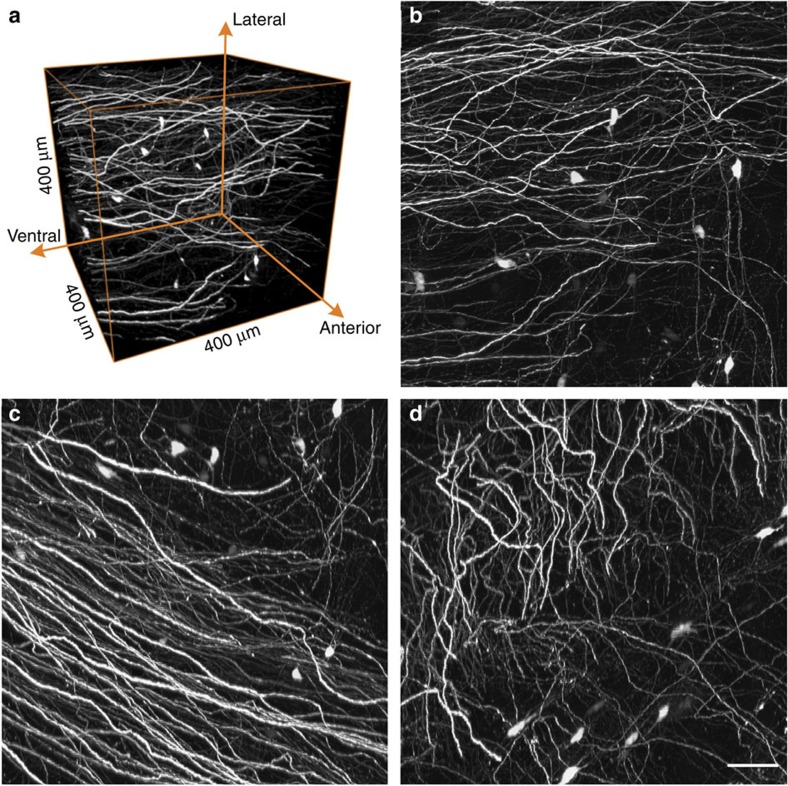
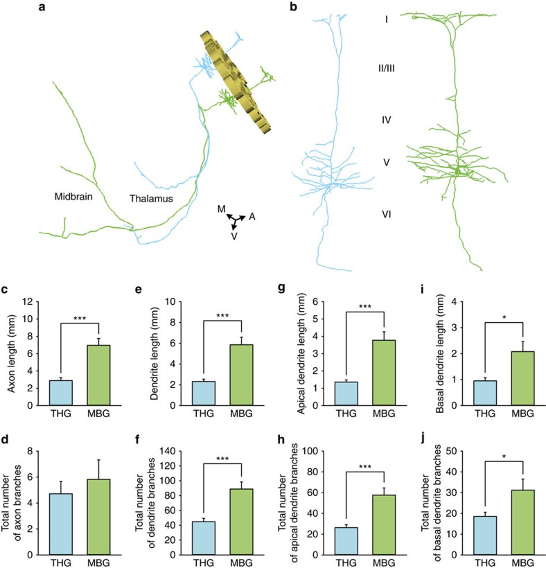
The precise annotation and accurate identification of neural structures are prerequisites for studying mammalian brain function. The orientation of neurons and neural circuits is usually determined by mapping brain images to coarse axial-sampling planar reference atlases. However, individual differences at the cellular level likely lead to position errors and an inability to orient neural projections at single-cell resolution. Here, we present a high-throughput precision imaging method that can acquire a co-localized brain-wide data set of both fluorescent-labelled neurons and counterstained cell bodies at a voxel size of 0.32 × 0.32 × 2.0 μm in 3 days for a single mouse brain. We acquire mouse whole-brain imaging data sets of multiple types of neurons and projections with anatomical annotation at single-neuron resolution. The results show that the simultaneous acquisition of labelled neural structures and cytoarchitecture reference in the same brain greatly facilitates precise tracing of long-range projections and accurate locating of nuclei.

Figure 1. Principle of BPS.

(a) BPS Data acquisition overview. The resin-embedded sample moves between the SIM and the microtome. The SIM acquires three raw images to reconstruct an optical section and axially scans for Z-stack imaging over a certain range. The entire coronal section is imaged in a mosaic manner. (b) Schematic representation of the real-time cytoarchitecture staining. The dye molecules penetrate into the fresh resin-embedded sample surface and immediately combine with the nucleic acids inside the cell body. The soma is then visualized.

Figure 2. Brain-wide dual-colour imaging of a Thy1-GFP M-line mouse brain.

(a,b) Maximum intensity projections of the coronal sections. The projections were 400 (a) and 1 μm (b) thick. (c) Merged images indicated by the white boxes in a,b. (d) An enlarged view of the area indicated by the upper white square in c, demonstrating the visualization of axonal boutons, indicated using arrowheads. (e) An enlarged view of the area indicated by the white rectangle in c demonstrating visualization of dendritic spines, indicated using arrowheads. (f,g) Raw signals of the enlarged views of the area indicated by the lower white square in c. (h) Merged image, demonstrating accurate co-localization at single soma resolution using PI staining. (c,h) The projection thicknesses of GFP and PI were 400 μm and 1 μm, respectively. Scale bars, (a,b) 1 mm; (c) 50 μm; (d) 40 μm; (e) 5 μm; and (f–h) 10 μm.

Figure 3. Continuous neural projections with high resolution.

(a) 3D reconstruction of a GFP-labelled image block without preprocessing. The image block is selected from the same whole-brain data set of Fig. 2 and located in the thalamus. (b–d) Maximum intensity projections on transverse, sagittal and coronal sections, accordingly. Each projection depth is 400 μm. Scale bar, 50 μm.

Figure 4. Localization and reconstruction of pyramidal neurons in the Thy1-GFP M-line mouse barrel field.

(a) PI-channel volume rendering and the 220-μm-thick perspective projection of the barrel field of the right hemisphere, showing layer IV cytoarchitecture. Scale bar, 200 μm. (b) A reconstructed pyramidal neuron and associated cytoarchitecture reference. (left) Neuron and the local layer IV cytoarchitecture of the D3 and D4 columns (410 × 340 × 80 μm image stack). The apical dendrites of this neuron are located in the barrel hollow of D3. The blue arrow indicates the location where the neuron passes through the upper boundary of the image stack. (right) The cytoarchitecture from layer I to the corpus callosum surrounding the same neuron as shown on the left. The blue arrowheads indicate barrel walls. Image stack volume size: 760 × 850 × 150 μm. Scale bar, 100 μm. (c) 3D reconstruction of the barrel walls and 50 representative neurons located in the barrel field. The barrel walls were reconstructed according to PI-stained images and represented as gold loops (height: 80 μm). (d) The distribution of all long-range projection neurons among the 50 representative neurons. The thalamus, midbrain and medulla are the major projection regions. L, left; P, posterior; and V, ventral. (e) Ten reconstructed neurons (c) and corresponding barrel columns. The five neurons shown on the left are long-tufted pyramidal neurons, and the remaining five neurons are short-sparse neurons. The orange neuron located in D3 is the same neuron shown in b. Blue, green and orange colours represent neurons with axons extending the furthest to the striatum or thalamus, the midbrain and the pons or medulla, respectively. Pink denotes local projection neurons.

Figure 5. Quantitative comparison of the fine morphology of neurons.

(a) 3D reconstruction of the barrel walls and two representative long-range projection neurons located in the barrel cortex. The barrel walls were reconstructed according to PI-stained images and represented as gold loops (height: 80 μm). The blue neuron was localized to the D5 barrel column and projected to the thalamus. The green neuron was localized in the E2 barrel column and projected to the midbrain. A, anterior; M, middle; and V, ventral. (b) The enlarged views of the dendrites of the two neurons in (a) showing the distinct dendrite complexities of the projection neurons in the two groups. (c,d) Histograms of the axonal lengths (P<0.001) and branch numbers (P=0.520) of the long-range neurons, respectively. THG (n=15) and MBG (n=11) represent the neurons projecting to the thalamus and midbrain, respectively. (e,f) Histograms of the dendrite lengths (P<0.001) and branch numbers (P<0.001) of long-range neurons, respectively. (g,h) Histograms of the apical dendrite lengths (P<0.001) and branch numbers (P<0.001) of long-range neurons, respectively. (i,j) Histograms of the basal dendrite lengths (P=0.017) and branch numbers (P=0.045) of long-range neurons, respectively. We performed Student's t-test on two groups by SPSS 22. Error bars were defined as s.e.m. Confidence level was set to 0.05 (P value). * represents P<0.05, and *** represents P<0.001.

Figure 6. Anterograde tracing and localization of brain-wide neural projections.

(a) Anterograde projections of AAV-GFP-labelled Cg neurons in the entire brain. The inset shows the main pattern of the Cg projecting to the whole brain, and the 15 passing regions are indicated in the global observation at low resolution. The grey sphere indicates the injection site. (b) Merged local maximum intensity projections of the sagittal planes of the corresponding positions indicated in a. Passing regions: (b1) corpus callosum, (b2) caudate putamen, (b3) primary/secondary motor cortex, (b4) anteroventral thalamic nucleus and anterodorsal thalamic nucleus, (b5) anteromedial thalamic nucleus and paratenial thalamic nucleus, (b6) ventromedial thalamic nucleus, zona incerta dorsal part (ZID), zona incerta ventral part (ZIV), and reticular thalamic nucleus, (b7) primary/secondary visual cortex, (b8) inferior colliculus (ic), (b9) mediodorsal thalamic nucleus central part, mediodorsal thalamic nucleus dorsal part and mediodorsal thalamic nucleus lateral part, (b10) periaqueductal gray, (b11) medial lemniscus and ZID, (b12) ZID/ZIV and cerebral peduncle, (b13) ic, (b14) superior colliculus and (b15) entorhinal cortex. The size of each panel is 300 × 320 μm. Green represents the maximum intensity projections of GFP-labelled axons. The projection thickness shown in images 3, 5, 6, 9, 13 and 14 is 32 μm, and the projection thickness of the other images is 64 μm. Magenta represents PI-stained cells (2 μm thickness). (c) Projection pattern from Cg neurons on the coronal plane indicated with an arrow in (a). Green represents the maximum intensity projection of GFP-labelled projections (960 μm total thickness). Magenta represents PI-stained cells (2 μm thickness). The inset is an amplified image of the block shown in (c) containing sparse axons. (d) The reconstructed and localized axon indicated with arrowheads in (c). The cell body is located in the Cg region, and the axon connects to DpWh. Additionally, the axon bifurcates in the ic and LPMR brain regions. Purple represents the PI-counterstained cytoarchitecture background. Scale bar, 50 μm (b); 500 μm (c); 50 μm (the inset in c); and 100 μm (d).

Figure 7. Whole-brain imaging of GFP-labelled neurons in a SOM Cre-line mouse brain.

(a–e) Maximum intensity projections of different coronal sections showing the projection patterns with cytoarchitectonic references. The inset shows locations of images shown in a–e. The projection thicknesses of GFP-signal were 60 μm (a,b), 120 μm (c) 200 μm (d) and 100 μm (e). Magenta represents PI-stained cells (2 μm thickness). (f–i) Representative raw images showing the fine structure, such as axon boutons, of the long-range projections shown in (e). Scale bar, 1 mm (a–e) and 15 μm (f–i).

Figure 8. Reconstruction of sparse-labelled brainstem neurons with long-range projections.

(a) Maximum intensity projections of the coronal sections. The projection thickness was 900 μm. (b–g) Enlarged views of the single axon arbor and axon terminals of the neurons shown in a. The reconstructed boutons are indicated as white arrowheads. The large axon terminals were indicated as orange arrowheads. Scale bar, 1 mm (a); 100 μm (d); 50 μm (f); and 25 μm (b,c,e,g).

References

1. Li A. et al.. Micro-optical sectioning tomography to obtain a high-resolution atlas of the mouse brain. Science 330, 1404–1408 (2010). - PubMed
1. Ragan T. et al.. Serial two-photon tomography for automated ex vivo mouse brain imaging. Nat. Methods 9, 255–258 (2012). - PMC - PubMed
1. Gong H. et al.. Continuously tracing brain-wide long-distance axonal projections in mice at a one-micron voxel resolution. Neuroimage 74, 87–98 (2013). - PubMed
1. Wickersham I. R. et al.. Monosynaptic restriction of transsynaptic tracing from single, genetically targeted neurons. Neuron 53, 639–647 (2007). - PMC - PubMed
1. Hezel M., Ebrahimi F., Koch M. & Dehghani F. Propidium iodide staining: a new application in fluorescence microscopy for analysis of cytoarchitecture in adult and developing rodent brain. Micron 43, 1031–1038 (2012). - PubMed
Publication types