Optical imaging of individual biomolecules in densely packed clusters

Abstract

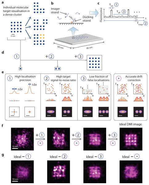
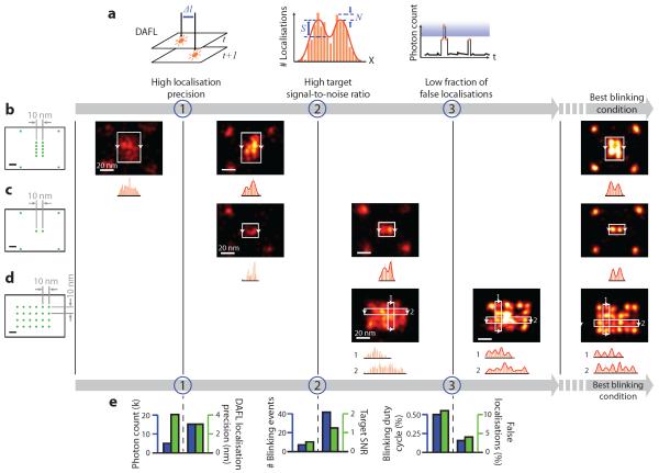
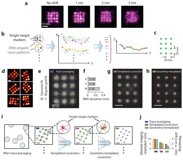
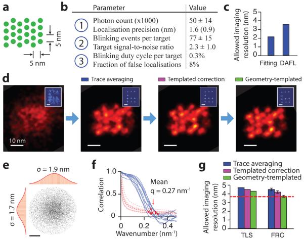
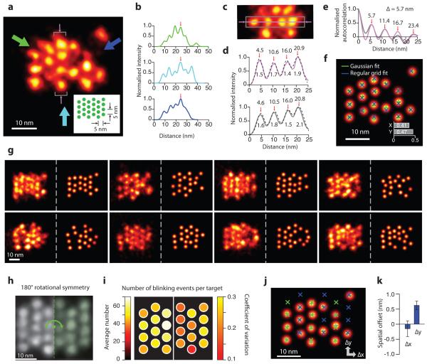
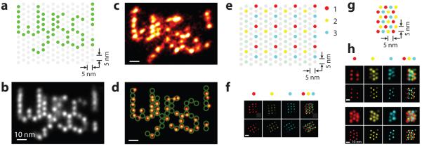
Recent advances in fluorescence super-resolution microscopy have allowed subcellular features and synthetic nanostructures down to 10-20 nm in size to be imaged. However, the direct optical observation of individual molecular targets (∼5 nm) in a densely packed biomolecular cluster remains a challenge. Here, we show that such discrete molecular imaging is possible using DNA-PAINT (points accumulation for imaging in nanoscale topography)-a super-resolution fluorescence microscopy technique that exploits programmable transient oligonucleotide hybridization-on synthetic DNA nanostructures. We examined the effects of a high photon count, high blinking statistics and an appropriate blinking duty cycle on imaging quality, and developed a software-based drift correction method that achieves <1 nm residual drift (root mean squared) over hours. This allowed us to image a densely packed triangular lattice pattern with ∼5 nm point-to-point distance and to analyse the DNA origami structural offset with ångström-level precision (2 Å) from single-molecule studies. By combining the approach with multiplexed exchange-PAINT imaging, we further demonstrated an optical nanodisplay with 5 × 5 nm pixel size and three distinct colours with <1 nm cross-channel registration accuracy.

Figure 1. Principle and requirements of discrete molecular imaging (DMI)

(a) Concept of super-resolution discrete molecular imaging, illustrated with point array representation (blue points represent individual molecular targets, yellow points represent chemical modifications). Left, a regular 16-component biomolecular complex; right, its various forms of structural and chemical variations. (b) Illustration of DNA-PAINT principle: transient binding between a docking strand and dye-conjugated imager strands (top), illustrated on a synthetic DNA origami nanostructure, where each cylinder represents a DNA double helix (bottom). (c) Schematic DNA-PAINT blinking time trace of a single imaging target. Three blinking characteristics measure (1) blinking on-time, τ_on, (2) total imaging time, Timage and (3) blinking off-time, τ_off, and can be tuned to meet the three blinking requirements in (e). (d) Schematics of different substructures from the complex in (a): a single target, a pair of close-by targets, and a dense lattice, which need different blinking requirements in (e) to be clearly visualised. (e) Technical requirements for achieving discrete molecular imaging. Each panel outlines one technical requirement, and depicts schematically the effect on imaging quality before (left column) and after (right column) the requirement is satisfied. For each condition, intensity profile in 1D (top), fitted Gaussian centres in 1D (middle) and 2D (bottom) are shown for requirement (1); localisation time trace in 1D (top), localisation histogram in 1D (middle) and 2D (bottom) are shown for requirements (2), (3) and (*). Orange lines and crosses indicate localisations. Orange bars depict localisation histograms. Solid red lines and dotted grey lines indicate successful and failed Gaussian fittings on localisation histograms, respectively. In panel 3, grey crosses indicate true localisations eclipsed by false double-blinking localisations. The same numbering for technical requirements (1)-(3) is also used in Fig. 2 and 4, and Supplementary Figure S2. (f-g) Simulations of imaging effects of the technical requirements for the complex in (a), under increasingly better imaging conditions without stage drift (f), or under non-ideal imaging conditions with one of the four requirements unsatisfied (g). See online methods and Supplementary Methods S2 for simulation details, and Supplementary Notes S7 for discussions. Scale bars: schematic length scale 5 nm in (a) and (e), 10 nm in (f) and (g).

Figure 2. Systematic characterisation of blinking requirements and optimisation of DNA-PAINT imaging quality

(a) Methods for systematic characterisation of the three blinking requirements depicted in Fig. 1. (1) Distance between adjacent-frame localisations (DAFL) measures distance between pairs of spatially-close localisations originated from adjacent camera frames. (2) Target signal-to-noise ratio (target SNR) measures separability of peaks in localisation histogram, in the super-resolved image. S, signal; N, noise; red curve indicates two-peak Gaussian fit. (3) Photon count cut-off in blinking trace measures fraction of false localisations. Blue shaded area indicates identified false localisations. Orange markers, bars and curves indicate localisations, histograms and time traces, respectively. (b-d) Designed origami standards with 10 nm spacing under different blinking conditions. Leftmost column, design schematics of DNA origami standards; green dots indicate DNA-PAINT docking strands; four corners in (b) and (c) are used as alignment markers. Right five columns, DNA-PAINT images under increasingly better blinking conditions (one condition per column). Histograms below images show projection profiles from the areas indicated by white boxes and projected along the directions of arrows. (e) Quantitative characterisation and pairwise comparisons of imaging conditions used in (b-d), before and after meeting each additional requirement, assayed with methods in (a). For each comparison, left axis (blue) shows the control parameter and right axis (green) shows experimental measurement. For more details, see Supplementary Figures S3-S5 on origami designs, Supplementary Figures S6-S13 for super-resolution images, online methods and Supplementary Methods S3, S5 for DNA-PAINT imaging conditions and analysis methods. Scale bars, 10 nm in schematics and 20 nm in super-resolution images.

Figure 3. Principle and performance of DNA nanostructure templated drift correction

(a) Effect of drift on imaging quality, simulated for the biomolecular complex in Fig. 1a with 1 nm localisation precision and different levels of stage drift. Only with 1 nm (r.m.s.) or less drift can the structure be clearly visualised. (b) Principle of templated drift correction method with pre-designed nanostructure patterns. Illustrated with a three-target marker example, schematics show nano-pattern design with single-target markers (left), localisation time traces from individual single-target markers (middle), and averaged drift correction trace after combining traces from many markers (right). Targets and traces are colour-matched. (c) Design schematics of a 3 × 4 square grid with 20 nm point-to-point spacing on a DNA origami nanostructure. Each green dot indicates a docking strand. (d) Representative DNA-PAINT super-resolution images of the 20 nm grid structure in (c), imaged with 300 ms frame time, 30,000 total frames, and 3 nM imager strands. Missing grid points were likely due to synthesis or incorporation defects (see Supplementary Notes S9.1 for more discussions). (e) Single-particle averages of 20 nm grid images (N = 700) after trace averaging. Overlaid crosses indicate Gaussian fitted centres (red) and regular grid-fitted centres (green) using the red crosses as fitting targets. (f) Root-mean-square (r.m.s.) deviation between the Gaussian fitted and regular grid-fitted centres in (e). (g, h) Single-particle averages of 20 nm grid images (N = 700) after templated (g) and geometry-templated (h) drift correction. Overlaid crosses indicate Gaussian fitted (red) and regular grid-fitted centres (green) as in (e). The same colour code for different stages of drift correction in (e), (g), (h) are also used in (i), (j) and Fig. 4. (i) Procedure for templated and geometry-templated drift correction with 20 nm grid structures as templates. Schematics shows a large field-of-view image with many drift markers, after simple trace averaging (leftmost). Each grey circle indicates a 20 nm drift marker. Zoomed-in (square) schematics shows a super-resolved 20 nm grid marker, after simple trace averaging (left), after templated drift correction (middle), and after geometry-templated correction (right). Further zoomed-in schematics (round) shows one single-target marker and calculation of offset vectors. In zoomed-in schematics (square and round), grey dots indicate localisations, green dots and lines indicate Gaussian-fitted centres and regular grid-fitted lattices as guides for templated and geometry-templated drift correction calculation, red line segments with arrowheads represent calculated offset vectors. (j) Comparison of allowable imaging resolution (measured in FWHM, blue) and estimated remaining drift (green) at different stages of drift correction. For more details, see online methods and Supplementary Methods S2, S5 for simulation and analysis methods, Supplementary Figures S14 for super-resolution images. Scale bars: 10 nm in (a), 20 nm in (d-f) and zoomed-in images in (i).

Figure 4. Systematic quality analysis of 5 nm grid super-resolution image

(a) Design schematics of a 4 × 6 triangular grid structure with ~5 nm point-to-point spacing on a DNA origami nanostructure. Each green dot indicates a docking strand. (b) Critical imaging quality parameters for the three blinking requirements. Localisation precision value in brackets was measured by single-molecule fitting uncertainty. (c) Allowable imaging resolution assayed by two methods before drift correction, single-molecule fitting uncertainty (Fitting) and distance between adjacent-frame localisations (DAFL), both estimated in FWHM. (d) Comparison of DNA-PAINT images of a 5 nm grid structure and a 20 nm grid drift marker (blue, inset) at different stages of drift correction. (e, f) Measured imaging resolution assayed by two methods after drift correction. (e) Target localisation spread (TLS). The point cloud shows overlapped localisations from individually separable targets and aligned by centre of mass. Histograms are shown for horizontal (left) and vertical (top) projections. Red curves indicate Gaussian fit. (f) Fourier ring correlation (FRC). Correlation curves (blue, solid lines) and noise-based cutoff (red, dotted lines) are shown for 10 representative images; red dots indicate crossing points. (g) Comparison of measured imaging resolution at different stages of drift correction, assayed by TLS and FRC. Red dashed line indicates localisation precision-limited best allowable resolution (as determined by DAFL). DNA-PAINT imaging conditions used for this experiment: 400 ms frame time, 40,000 total frames, and 1 nM imager strand concentration. See online methods, Supplementary Figures S15-S19 and Methods S3, S5 for more details on assay methods and results. Scale bars, 10 nm in images, 20 nm in insets in (d), 2 nm in (e).

Figure 5. Discrete molecular imaging of 5 nm grid structure

(a) Representative DMI image of a 5 nm triangular grid structure obtained with DNA-PAINT. Inset shows design schematics, where each green dot indicates a docking strand. Arrows indicate projection directions and areas of study for panels (b-e). Missing grid points were likely due to synthesis or incorporation defects (see Supplementary Notes S9.1 for more discussions). (b) Intensity projection profiles from the image in (a), along the directions indicated by colour-matched arrows. Profiles are aligned by central peaks indicated by red arrows. (c) Cropped-out image from (a), showing central region (grey rectangle) and central pixel line (magenta line and arrows) used for analysis in (d, e), also marked by grey brackets and thin magenta arrows in (a). (d) Intensity profile along the central line (magenta), and projection from the central region (grey), as indicated by colour-matched regions in (c), and four-peak Gaussian fit for both (black, dashed lines). Numbers indicate fitted centre positions and standard deviation values for each peak, with an average of 1.7 nm, supporting a 4.0 nm FWHM resolution. (e) Auto-correlation analysis from colour-matched profiles in (d), showing consistent periodicity of 5.7 nm. (f) Automatic multi-target fit of the 5 nm grid image in (a). Overlaid crosses indicate Gaussian-fitted centres (green) and regular grid-fitted centres using the green crosses as targets (blue). Inset shows r.m.s. deviation between the green and blue crosses (<0.5 nm in 1D and <0.7 nm in 2D). (g) More representative images of the 5 nm grid structures, showing structural regularity and heterogeneity. For each structure, left panel shows super-resolution rendered image, right panel shows automatic fitted image. (h) Single-particle class average of the 5 nm grid (N = 25). Green dashed line and arrow indicate symmetry axis and operation of the structure. (i) Uniformity of blinking kinetics, as represented on a 5 nm degenerate grid. colour maps show averages (left) and coefficients of variation (right) of the number of blinking events for each distinguishable target. (j) Automatic multi-target fit (grey) and two-component grid fit of 5 nm image in (a), allowing an offset between two groups of targets with opposite staple strand orientations, coloured in green and blue respectively. (k) Offsets between the two groups of staples in (j) measured from single-molecule images, error bars indicate standard deviation (N = 10). It is important to note that no prior knowledge of the sample structure (the 5 nm grid) was used to produce the above results. DNA-PAINT imaging condition used for this experiment: 400 ms frame time, 40,000 total frames, and 1 nM imager strand concentration. See Supplementary Figures S15, S20-S22 and Methods S5, S6 for super-resolution images and analysis details, and Supplementary Notes S9 for discussions. Scale bars: 10 nm in all panels.

Figure 6. Discrete molecular imaging with complex patterns and multiplexed visualisation

(a-d) DMI of a five-character pattern “Wyss!” on a DNA origami nano-display board with 5 nm pixel size. (a) Design schematics. Each dot indicates a staple strand. Green dots were extended with DNA-PAINT docking strands. (b) Single-particle class average of the “Wyss!” pattern (N = 85). (c) Representative single-molecule image of the “Wyss!” pattern under DMI. (d) Overlay of the design schematics on top of automatically fitted single-molecule image in (c). (e-h) Three-colour multiplexed DMI, each colour indicates a separate imaging channel with an orthogonal DNA-PAINT sequence. (e) Design schematics of a three-colour dual-purpose drift and alignment marker. (f) Cross-channel alignment. Thee single-channel images (left three columns) and one composite image (rightmost column) are shown for two example alignment markers. (g) Design schematics of a three-colour 5 nm grid structure. (h) Representative multiplexed DMI image of three-colour 5 nm grid pattern as in (g). DNA-PAINT super-resolution images (top row) and automatically fitted image (bottom row) are shown for all three single-colour channels (left three columns) and the combine image (rightmost column), for two representative 5 nm grid structures. DNA-PAINT imaging conditions used in these experiments are as follows. “Wyss!” letter pattern image: 500 ms frame time, 100,000 total frames, and 0.4 nM imager strand concentration. Multi-colour pattern image: 400 ms frame time, 2-3 nM imager strand concentration, 20,000 total frames for each colour channel. See Supplementary Figures S23, S24 for more super-resolution images, online methods and Supplementary Methods S5, S6 for image analysis methods. Scale bars: 10 nm in (b-d), 20 nm in (f), and 10 nm in (h).

References

1. Hell SW, Wichmann J. Breaking the diffraction resolution limit by stimulated emission: stimulated-emission-depletion fluorescence microscopy. Optics Letters. 1994;19 - PubMed
1. Klar TA, Hell SW. Subdiffraction resolution in far-field fluorescence microscopy. Optics letters. 1999;24:954–956. - PubMed
1. Gustafsson MG. Surpassing the lateral resolution limit by a factor of two using structured illumination microscopy. Journal of microscopy. 2000;198:82–87. - PubMed
1. Gustafsson MG. Nonlinear structured-illumination microscopy: wide-field fluorescence imaging with theoretically unlimited resolution. Proceedings of the National Academy of Sciences of the United States of America. 2005;102:13081–13086. - PMC - PubMed
1. Betzig E, et al. Imaging intracellular fluorescent proteins at nanometer resolution. Science (New York, N.Y.) 2006;313:1642–1645. - PubMed
Publication types