Downscaled and debiased climate simulations for North America from 21,000 years ago to 2100AD

Abstract

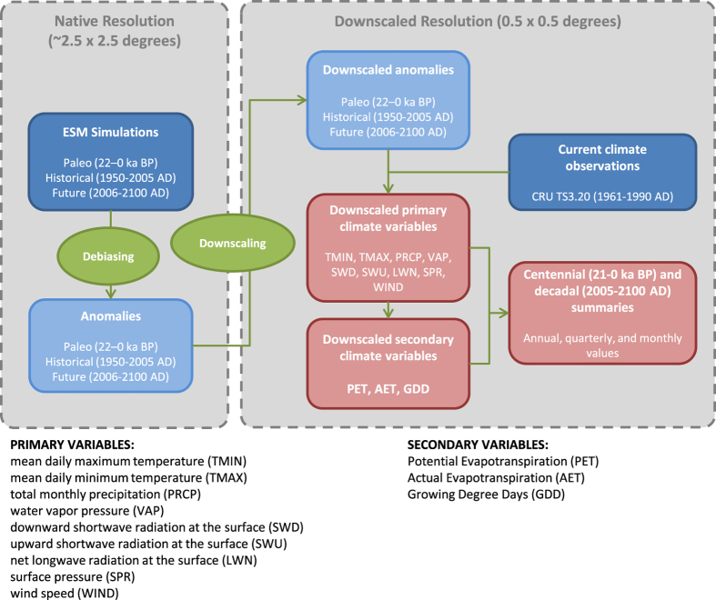
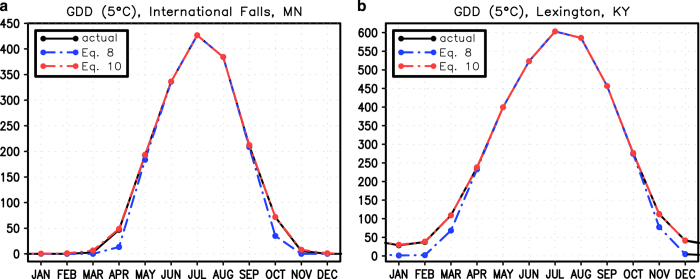
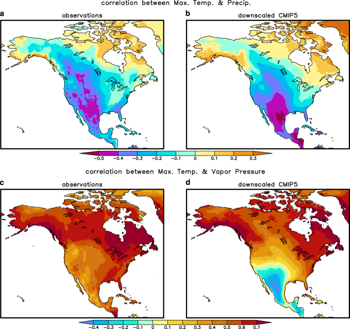
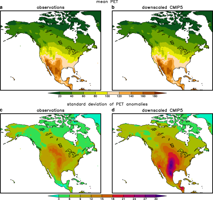
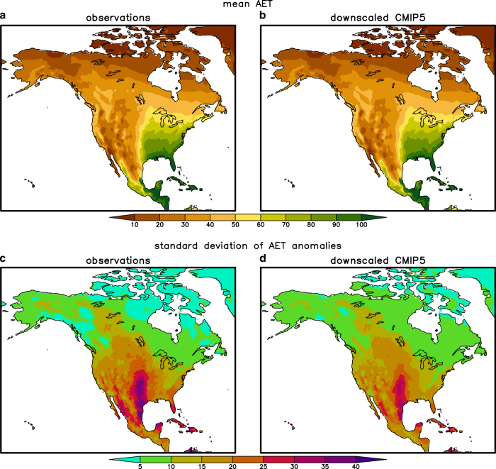
Increasingly, ecological modellers are integrating paleodata with future projections to understand climate-driven biodiversity dynamics from the past through the current century. Climate simulations from earth system models are necessary to this effort, but must be debiased and downscaled before they can be used by ecological models. Downscaling methods and observational baselines vary among researchers, which produces confounding biases among downscaled climate simulations. We present unified datasets of debiased and downscaled climate simulations for North America from 21 ka BP to 2100AD, at 0.5° spatial resolution. Temporal resolution is decadal averages of monthly data until 1950AD, average climates for 1950-2005 AD, and monthly data from 2010 to 2100AD, with decadal averages also provided. This downscaling includes two transient paleoclimatic simulations and 12 climate models for the IPCC AR5 (CMIP5) historical (1850-2005), RCP4.5, and RCP8.5 21st-century scenarios. Climate variables include primary variables and derived bioclimatic variables. These datasets provide a common set of climate simulations suitable for seamlessly modelling the effects of past and future climate change on species distributions and diversity.

Figure 1. Workflow diagram summarizing the major steps used to generate the debiased and downscaled paleoclimate and 21st-century datasets described here.

The primary climate variables are first debiased by differencing (or similar calculation, see Section 3) each paleoclimate or future climate simulation from a climate simulation representing present climates. These anomalies (also known as factors) are then downscaled via bilinear interpolation to a higher-resolution grid corresponding to the resolution of the modern observational dataset. The anomalies are then added to (or multiplied by, see Section 3) the observational data to produce the downscaled primary variables. From these downscaled primary variables, secondary bioclimatic variables (GDD, AET, PET) are calculated. Finally, statistical summaries of all variables are calculated at centennial (paleoclimatic simulations) and decadal resolution (21st-century projections).

Figure 2. Anomaly maps showing examples of the downscaled differences between simulated past and future climates to the 20th century baselines.

Top row: difference maps for mean maximum daily temperature, for 21 ka BP, 11 ka BP, 6 ka BP and 2071–2100AD. The paleosimulations are for the downscaled SynTrace CCSM3 simulation, with locations under the ice sheet masked out. The upper-right plot is the difference between 2071–2100 and 1950–2005, averaged over 12 climate models and for the RCP8.5 scenario. Second row: as top row, but for the percent change in precipitation compared to present. Third row: as top row, but for growing degree days (GDD) base 5C. Fourth row: as top row, but for the ratio of mean annual AET to mean annual PET.

Figure 3. Assessment of the process used to predict the monthly annual cycle from the seasonal annual cycle for temperature.

This plot shows maximum or minimum temperature annual cycle for Madison, WI ((a) and (b)) and a point northwest of Oaxaca, Mexico ((c) and (d)). The observed monthly annual cycle is in black. The observed monthly annual cycle averaged together into seasonal means is in blue. The monthly annual cycle estimated from the seasonal means by simple linear interpolation is in green. The monthly annual cycle estimated from the seasonal means by the new method described in the text is in red.

Figure 4. Estimating the monthly annual cycle from the seasonal annual cycle for precipitation.

Shown is the precipitation annual cycle for (a) Madison, WI, (b) a point northwest of Oaxaca, Mexico, (c) a point in northwest Mexico, and (d) a point 4° north in Arizona. The observed monthly annual cycle is in black. The observed monthly annual cycle averaged together into seasonal means is in blue. The monthly annual cycle estimated from the seasonal means by linear interpolation is in green. The monthly annual cycle estimated from the seasonal means by the new method described in the text is in red.

Figure 5. Estimating the monthly annual cycle of GDD base 5° using the monthly mean temperature only(blue) and the monthly mean temperature and the daily standard deviation (red).

The actual GDD is in black. (a) International Falls, MN, (b) Lexington, KY.

Figure 6. Maps of the temporal correlation between monthly anomalies for selected climate variables, to check whether the downscaled dataset has preserved the correlational structure in observational data.

(a) Observed correlation between maximum temperature and precipitation (1950–2005). (b) As in (a) but for the downscaled CMIP5 data. This is the mean correlation averaged over 12 climate models. (c,d) As (a,b) but for maximum temperature and vapour pressure. The cross-correlation structure between temperature and precipitation is generally well-preserved, while the cross-correlation structure is less well preserved for vapour pressure.

Figure 7. Comparison of observed and downscaled simulated potential evapotranspiration (PET), represented as annual averages of monthly data.

(a) PET derived from observed variables such as temperature and vapour pressure. (b) As in (a) but for an average of 12 downscaled CMIP5 models. (c) Standard deviation of PET anomalies calculated from observational data. (d) As in (c) but for the downscaled CMIP5 models.

Figure 8. As Fig. 7, but for actual evapotranspiration (AET).

(a) AET derived from observed variables such as temperature and vapour pressure. (b) As in (a) but for an average of 12 downscaled CMIP5 models. (c) Standard deviation of AET anomalies calculated from observational data. (d) As in (c) but for the downscaled CMIP5 models.

References

Data Citations
1. Lorenz D. J., Nieto-Lugilde D., Blois J. L., Fitzpatrick M. C., Williams J. W. 2016. Dryad Digital Repository. http://dx.doi.org/10.5061/dryad.1597g - DOI
1. Moritz C. & Agudo R. The future of species under climate change: Resilience or decline? Science 341, 504–508 (2013). - PubMed
1. Fritz S. A. et al. Diversity in time and space: wanted dead and alive. Trends Ecol. Evol. 28, 509–516 (2013). - PubMed
1. Blois J. L., Zarnetske P. L., Fitzpatrick M. C. & Finnegan S. Climate change and the past, present, and future of biotic interactions. Science 341, 499–504 (2013). - PubMed
1. Jackson S. T. & Blois J. L. Community ecology in a changing environment. Proceedings of the National Academy of Sciences 112, 4915–4921 (2015). - PMC - PubMed
1. Kidwell S. M. Biology in the Anthropocene: Challenges and insights from young fossil records. Proceedings of the National Academy of Sciences 12, 4922–4929 (2015). - PMC - PubMed
Publication types