Water: A Tale of Two Liquids

Abstract

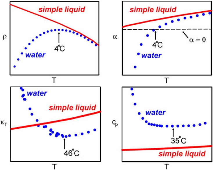
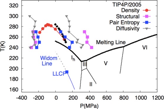
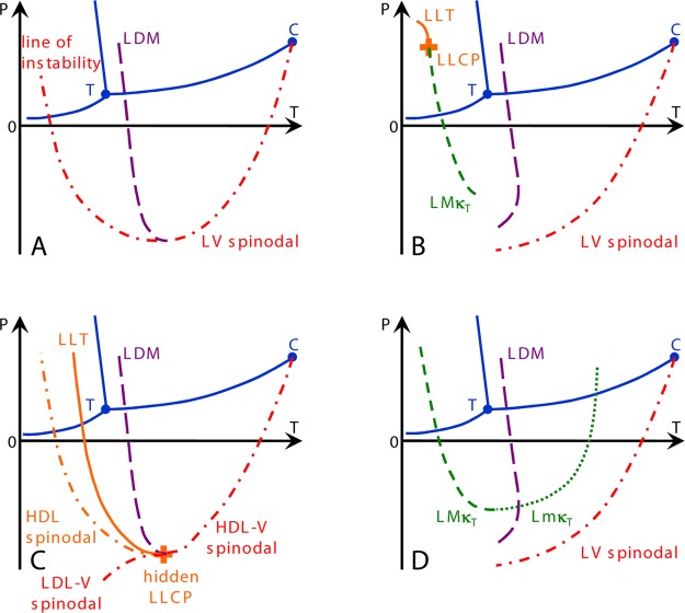
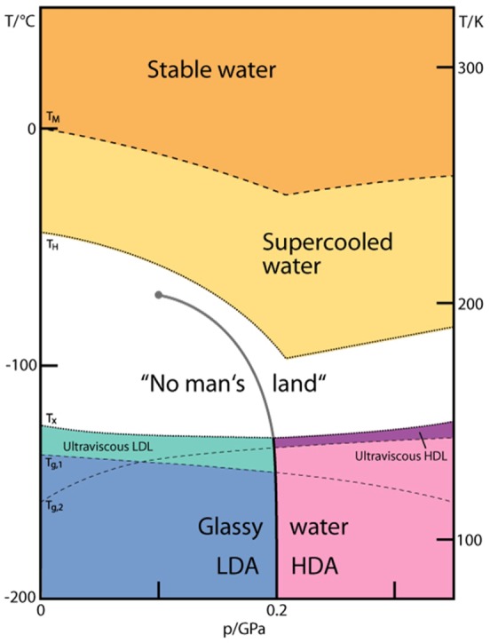
Water is the most abundant liquid on earth and also the substance with the largest number of anomalies in its properties. It is a prerequisite for life and as such a most important subject of current research in chemical physics and physical chemistry. In spite of its simplicity as a liquid, it has an enormously rich phase diagram where different types of ices, amorphous phases, and anomalies disclose a path that points to unique thermodynamics of its supercooled liquid state that still hides many unraveled secrets. In this review we describe the behavior of water in the regime from ambient conditions to the deeply supercooled region. The review describes simulations and experiments on this anomalous liquid. Several scenarios have been proposed to explain the anomalous properties that become strongly enhanced in the supercooled region. Among those, the second critical-point scenario has been investigated extensively, and at present most experimental evidence point to this scenario. Starting from very low temperatures, a coexistence line between a high-density amorphous phase and a low-density amorphous phase would continue in a coexistence line between a high-density and a low-density liquid phase terminating in a liquid-liquid critical point, LLCP. On approaching this LLCP from the one-phase region, a crossover in thermodynamics and dynamics can be found. This is discussed based on a picture of a temperature-dependent balance between a high-density liquid and a low-density liquid favored by, respectively, entropy and enthalpy, leading to a consistent picture of the thermodynamics of bulk water. Ice nucleation is also discussed, since this is what severely impedes experimental investigation of the vicinity of the proposed LLCP. Experimental investigation of stretched water, i.e., water at negative pressure, gives access to a different regime of the complex water diagram. Different ways to inhibit crystallization through confinement and aqueous solutions are discussed through results from experiments and simulations using the most sophisticated and advanced techniques. These findings represent tiles of a global picture that still needs to be completed. Some of the possible experimental lines of research that are essential to complete this picture are explored.

Figure 1

Anomalous thermodynamic properties of water compared to simple liquids. Schematic comparison of the isobaric temperature dependence of the density ρ, thermal expansion coefficient α_P, isothermal compressibility κ_T, and isobaric heat capacity, C_P, for water and a simple liquid. Reproduced with permission from ref (4). Copyright 2003 by IOP Publishing.

Figure 2

Thermodynamics of the condensed phases of water, illustrated for the TIP4P/2005 rigid-body model of water. Data for the phase boundaries are taken from ref (24). Boundaries of the structural, density, pair-entropy, and diffusivity anomalies are taken from ref (25). The experimental TMD line shown in filled black diamonds is taken from ref (26). The Widom line (see the definition in section 6) is taken from ref (27). Reproduced from ref (21) with permission from the PCCP Owner Societies.

Figure 3

Scenarios that might account for the behavior observed in Figure 1. (A) Speedy’s stability limit conjecture, (B) Poole et al.’s second critical point, (C) Poole et al.’s “weak bond”-modified van der Waals model, now the critical-point-free scenario, and (D) Sastry et al.’s singularity-free scenario. Continuous blue curves show the known equilibrium coexistence lines between liquid, solid, and vapor with the triple point marked as T. Liquid–vapor equilibrium terminates at the critical point C. The long-dashed purple line shows the line of density maxima (LDM), and the short-dashed and dotted green lines are the lines of isothermal compressibility maxima (LMκT) and minima (LmκT), respectively. Dash–dotted lines indicate lines of instability. In scenarios A and C, the LDM keeps a negative slope and ends at a line of instability. In scenarios B and D, the LDM reaches a maximum temperature and changes its slope, eventually merging with a line of density minima (not shown for clarity). When the scenario comprises a liquid–liquid transition, it is displayed with a continuous orange line (LLT), and the liquid–liquid critical point is shown as an orange plus. Adapted from ref (47). Copyright 2014 National Academy of Sciences.

Figure 4

Phase diagram of noncrystalline water (adapted from ref (75), courtesy of Stephan Fuhrmann and Thomas Loerting). No-man’s land indicates the region in which only crystalline ices have been observed so far. It is enclosed by the homogeneous crystallization line T_H from the top and the crystallization line T_X from the bottom. Two ultraviscous liquid domains, low- and high-density liquid water (LDL and HDL), can be found just below T_X. The two corresponding glass transition temperatures T_g,1 and T_g,2 separating the glassy solids LDA and HDA from the ultraviscous liquids LDL and HDL are taken from refs (76) and (77), respectively. Please note the metastable extension of T_g,1 into the stability region of HDA and of T_g,2 into the stability region of LDA/LDL. A first-order liquid–liquid phase transition line (LLPT) ends in the purported liquid–liquid critical point (LLCP).

Figure 5

Radial oxygen–oxygen pair-distribution functions for HDL and LDL demonstrating the structural difference between high- and low-density water at ambient temperature. Adapted with permission from ref (67). Copyright 2000 by the American Physical Society.

Figure 6

Pressure–temperature projection of the metastable phase behavior of the ST2b model for water from Liu et al. showing the liquid–liquid coexistence curve (black squares), the LDL spinodal (up triangles), and the HDL spinodal (down triangles). Solid and dashed lines are a guide to the eye, and the red circle is the critical point from ref (118). Reproduced with permission from ref (117). Copyright 2012 American Institute of Physics.

Figure 7

Free-energy surface of the ST2 model with vacuum boundary conditions at 228.6 K and 2.4 bar from Palmer et al. These conditions correspond to liquid–liquid equilibrium. Contours are spaced 1 k_BT apart. Reproduced with permission from ref (119). Copyright 2014 Macmillan Publishers Limited.

Figure 8

Low-density fraction from simulations of water-like models, and the predictions from the two-state thermodynamics (Reproduced with permission from ref (163). Copyright 2014 AIP Publishing LLC): (a) ST2(II) (denoted ST2b in Table 1), a version of the ST2 model. Fraction x is the low-density fraction. Symbols are simulation data. Solid curves are theoretical predictions. Dashed curve is a mean-field approximation. (b) mW model. Reproduced with permission from ref (136). Copyright 2013 AIP Publishing LLC. Solid curves are theoretical predictions which include clustering of water molecules with average aggregation number N = 6.

Figure 9

Density of cold and supercooled water as a function of temperature along isobars. Reproduced with permission from ref (39). Copyright 2012 MacMillan Publishers. Symbols represent experimental data.^,, Black curves are the predictions of the two-state model.T_M (dark red) indicates the melting temperature, and T_H indicates the homogeneous nucleation temperature. The thick blue line is the predicted liquid–liquid equilibrium curve, with the critical point C. The red line is the line of maximum density, and the green line is the line of a constant LDL fraction of about 0.12.

Figure 10

Optimization of the critical-point location (Reproduced with permission from ref (39). Copyright 2012 Macmillan Publishers Limited). For a given location of the critical point and a particular set of the adjustable parameters, the residual for each experimental data point is computed as the difference between the measured value and the computed value of that property. These individual residuals are made dimensionless by an experimental uncertainty and then summed, with the lowest value of the sum of squared residuals that can be achieved for each location of the critical point by varying the adjustable parameters. The solid red line is the hypothesized liquid–liquid transition curve. The dashed curve shows the temperature of homogeneous ice nucleation. The blue dotted curve is the liquid–liquid transition curve suggested by Mishima, and the green dotted curve is the singularity line suggested by Kanno and Angell.

Figure 11

Experimental O 1s soft X-ray emission spectra of gas-phase water, liquid water at different temperatures, and amorphous and crystalline ice, with an energy scale displaying the full spectrum (A) or only the lone-pair, 1b₁ region (B). The excitation energy is 550 eV, well above the ionization threshold. Peak components are labeled based on the molecular orbitals for a water molecule. The highest peak (1b₁) splits into double peaks (1b₁^′ and 1b₁^″). XES spectra of amorphous (−190 °C (83 K)) and crystalline ice from Gilberg et al. are included for comparison. Figure adapted with permission from ref (180). Copyright 2008 by Elsevier.

Figure 12

Ultrafast X-ray probing of water structure below the homogeneous ice nucleation using micrometer-sized water droplets falling in vacuum, Reproduced with permission from ref (178). Copyright 2014 Macmillan Publishers Limited. (a) Scattering structure factor, S(q). Data reveal a continuously increasing split of the principal S(q) maximum into two well-separated peaks, S₁ and S₂ (dashed lines). (b) Experimental tetrahedrality (g₂) values, derived from the measured split, Δq, between the two peaks in (a) as calibrated against a fit to molecular dynamics data. g₂ is the height of the second peak in the O–O pair-distribution function. Error bars are estimated from the maximum and minimum Δq values allowed by the uncertainty in the S₁ and S₂ peak positions. Also shown is the fourth-order polynomial least-squares fit to the experimental data (black solid line), where the last (that is, low-T) two data points for the 12 μm diameter droplets and the last data point for the 9 μm diameter droplets are ignored owing to high nonlinearity in the detector response (see ref (178)). For comparison, the temperature dependences of g₂ for the TIP4P/2005 (red dashed line) and SPC/E (purple dashed line) models are depicted along with the characteristic value of g₂ for LDA ice (blue dash-dotted line).

Figure 13

Two-state model for TIP4P/2005 water. (a) Values of the fraction of the locally favored S state (s) as a function of temperature for all simulated pressures. Symbols mark the values obtained by decomposition of the order parameter distribution, P(ζ), at the corresponding state point. Continuous lines are fits according to the two-state model. (b) Temperature dependence of density for several pressures. Continuous lines are simulation results, while symbols are obtained from the two-state model. Reproduced with permission from ref (216). Copyright 2014 Macmillan Publishers Limited.

Figure 14

Analysis of the inherent structure in simulations of TIP4P/2005 water. (A–C) Plot of the temperature-dependent distributions of LSI values at (A) 1, (B) 1000, and (C) 1500 bar. (D) Fraction of molecules in each distribution as a function of temperature and pressure. The Widom line (see the definition in section 6) at each pressure is indicated by a vertical line and corresponds to the crossing point between the high- and low-LSI distributions. Figure adapted with permission from ref (220). Copyright 2011 Royal Society of Chemistry.

Figure 15

Comparison of experimentally determined nucleation rates J of water using microdroplets (black hollow markers⁻ and red and brown filled dots), nanodroplets (blue hollow markers^,), thin films (green open diamonds and triangles,^, and hyperquenched water.^, Data of microdroplets (red solid line) and nanodroplets (blue symbols) follow different trajectories where the nanodroplet data might be affected by the large surface area to volume ratio and elevated internal pressure. An upper limit for the nucleation rate maximum within no-man’s land J_max (pink solid line) and a corresponding lower limit J_min (pink dashed line) were calculated from hyperquenching experiments on microdroplets.^,− The expected CNT behavior for a “fragile” (black dotted line) and a “strong” (green solid line) liquid are included as guides to the eye. We follow Jenniskens and Blake to obtain the “fragile liquid” CNT curve and also include an expected extension of the nucleation rate into no-man’s land (green curve) based on the requirement to lie between the upper and the lower limits from hyperquenched microdroplets. Figure adapted from ref (248). Copyright 2005 American Chemical Society.

Figure 16

Nucleation rate J as determined for the TIP4P/2005 model (blue solid line) compared to experiments (filled squares) of Pruppacher, Murray et al., and Manka et al. Experimental results from Laksmono et al. (filled circles) and Hagen et al. (filled triangles) were also included. The horizontal line corresponds to log₁₀J (cm^–3 s^–1) = 8, which is the approximate value of J at the homogeneous nucleation temperature in experiments (i.e., about 38 K below the melting point). Figure adapted with permission from ref (235). Copyright 2014 American Institute of Physics.

Figure 17

τ_x for ϕ = 0.7 for the TIP4P/2005 model as a function of the supercooling. τ_x is the time necessary to crystallize 70% of the system in an infinitely large system (blue line). (Inset) Plot of the nucleation time, τ_ν, versus the supercooling for systems having different numbers, N, of molecules of water. Figure reproduced with permission from ref (235). Copyright 2014 American Institute of Physics.

Figure 18

Isothermal compressibility of TIP4P/2005 water at 1 (blue), 70 (green), and 1200 bar (red) as a function of temperature. Symbols indicate the simulated values: squares (with error bars) obtained by Bresme et al. and circles (without error bars) obtained previously by Abascal and Vega. Curves represent values calculated from the two-structure equation of state. Figure reproduced with permission from ref (257). Copyright 2014 American Institute of Physics.

Figure 19

(Top) Crystal planes for the stable phases and ice 0. (Bottom left) Distribution of the average angle ⟨cos θ⟩ between the dipole moment of a molecule and its hydrogen-bonded neighbors for TIP4P/2005 water at T = 200 K and P = 1 bar in the liquid phase and the ice I_c, I_h, and ice 0 phases. (Bottom right) The same as in the left panel but for second-nearest neighbors. Adapted from ref (242). Copyright 2014 Macmillan Publishers Limited.

Figure 20

(Top) Snapshot of two configurations with the birth of a small crystalline nucleus (left) and a section of a nucleus of critical size (right). The color code is yellow for ice I_c, green for ice I_h, and magenta for ice 0. (Bottom) P–T phase diagram of mW water. Continuous lines indicate coexistence between the liquid phase and different crystal structures: ice I_h/I_c (blue), ice 0 (red), and clathrate CS-II (green). Dashed lines indicate constant chemical potential differences between the liquid and ice I_h/I_c (βΔμ = −0.721, in blue) and the liquid and ice 0 (βΔμ = −0.365, in red). The green dashed-dotted line is the I_c/CS-II coexistence line. Red open circles indicate state points where homogeneous nucleation is observed in simulations. Adapted from ref (242). Copyright 2014 Macmillan Publishers Limited.

Figure 21

Experimental IR results for structural change of confined water upon crossing the Widom line (Adapted with permission from ref (292). Copyright 2009 Macmillan Publishers Limited.). (a) Relative population of HDA-like and LDA-like water species as a function of temperature. (b) Derivative of the relative population for HDA-like and LDA-like water species. The maximal change occurs at the temperature T_max, where the Widom line is crossed.

Figure 22

Multiparticle correlation. Contributions to the entropy and the heat capacity anomaly. The total (C_P), pair (C₂), and triplet (C₃) contributions as a function of temperature (T) for the monatomic water (mW) model at 1 atm pressure. Reproduced with permission from ref (333). Copyright 2014 American Institute of Physics.

Figure 23

Pressure–temperature phase diagram of water. Reproduced with permission from ref (297). Copyright 2015 Elsevier. Colored areas are used to identify the different possible states for liquid water. The melting line of ice I_h is shown at positive pressure by a solid blue curve and its extrapolation to negative pressure by a dashed blue curve. Black crossed white squares show the experimental supercooling limit. They define the homogeneous nucleation line based on conventional experimental techniques (solid black curve), which is extrapolated here to negative pressure (dashed black curve). Recent experiments using fast cooling techniques can shift the nucleation line to lower temperatures (new border, purple curves); they are displayed as white triangles and circle. Isochores of TIP4P/2005 water for the two densities used in a recent experiment are shown by the thick red and black curves. Simulations of TIP4P/2005 water are performed to find the maximum of κ_T along several isobars (brown diamonds), defining the line of maxima in κ_T (brown curve), that might emanate from an LLCP (white plus symbol). Because the predictions of TIP4P/2005 are in satisfactory agreement with the reported experimental results in the supercooled region, this figure seems to indicate that the line of maxima in κ_T (and other extrema in the response functions) is not accessible to conventional experiments at positive pressure but might become accessible to fast cooling techniques at positive pressure or to conventional techniques but in the doubly metastable region at negative pressure.

Figure 24

Molecular dynamics simulations of water in MCM-41. In the picture we can see the difference between bound and free water which show distinct dynamical behavior and the behavior of the relaxation time of free water that shows the FTS transition that coincides with the Widom line (not shown). Reproduced with permission from ref (293). Copyright 2010 American Chemical Society.

Figure 25

Suppression of the anomaly of the heat capacity in aqueous solutions of sodium chloride (Reproduced with permission from ref (159). Copyright 2014 AIP Publishing LLC). Symbols: experimental data of Archer and Carter.^, Solid curves: predictions based on two-state thermodynamics. Dashed curve shows the positions of the melting temperatures. Dashed-dotted curve shows the temperatures of homogeneous ice formation.

Figure 26

Phase diagram of NaCl aqueous solutions of supercooled water as obtained from molecular dynamics simulations properly matched to the experimental data. Upon increasing salt content the LDL region shrinks and the LLCP is shifted to lower pressures and higher temperatures. Reproduced from ref (286). Copyright 2011 American Chemical Society.

Figure 27

FTS transition points (circles) and Widom line (continuous line) in a NaCl aqueous solution as obtained from molecular dynamics simulations. The nose-shaped line is the TMD, and the dashed line is the liquid–gas limit of mechanical stability. Reproduced with permission from ref (291). Copyright 2013 American Institute of Physics.

Figure 28

Comparison of the compressibility vs temperature relation at 0.1 MPa obtained with the TIP4P/2005 pair potential (heavy red curve) with the experimental findings and their extensions with decreasing temperature as follows: (first red point) −20 °C (253 K), combination of SAXS data (Huang et al.) and direct p–V data (Speedy and Angell) that are in close agreement; (second red point) −24 °C (249 K), lowest temperature direct measurement of Speedy and Angell; (dark green point) 239 K, limit of Holten and Anisimov extrapolation of ambient pressure fitted data; (light green point) 235 K, based on low-T limit of heat capacity measurements that follow the power law with divergence temperature of 226 K, essentially the same as for the compressibility.

Figure 29

(A) Fluorescent molecules whose intensities I_f have high sensitivity to pressure or viscosity. (B) Pressure dependence of the fluorescence intensity of molecule 1 in 1 M solution in acetone. Reproduced from ref (401) with permission. Copyright 2015 WILEY-VCH Verlag GmbH & Co.

Figure 30

(Left) Behavior of the isochores and the TMD with isochore density in the tuned S–W model with λ parameter = 23. The TMD does not reverse as it does for the silicon potential λ = 21. Flattened segments at lower temperatures correspond to broken ergodicity states (glasses on the simulation time scale). (Right) Isochores and density maxima behavior of the HGK equation of state for water.

References

1. Angell C. A. In Water: A Comprehensive Treatise; Franks F., Ed.; Plenum: New York, 1982; Vol. 7.
1. Debenedetti P. G.Metastable Liquids: Concepts and Principles; Princeton University Press: Princeton, 1996.
1. Franks F.Water: A Matrix of Life; Royal Society of Chemistry: Cambridge, 2000.
1. Debenedetti P. G. Supercooled and Glassy Water. J. Phys.: Condens. Matter 2003, 15, R1669–R1726. 10.1088/0953-8984/15/45/R01. - DOI
1. Debenedetti P. G.; Stanley H. E. Supercooled and Glassy Water. Phys. Today 2003, 56, 40–46. 10.1063/1.1595053. - DOI
Publication types
LinkOut - more resources