Inferring cortical function in the mouse visual system through large-scale systems neuroscience

Abstract

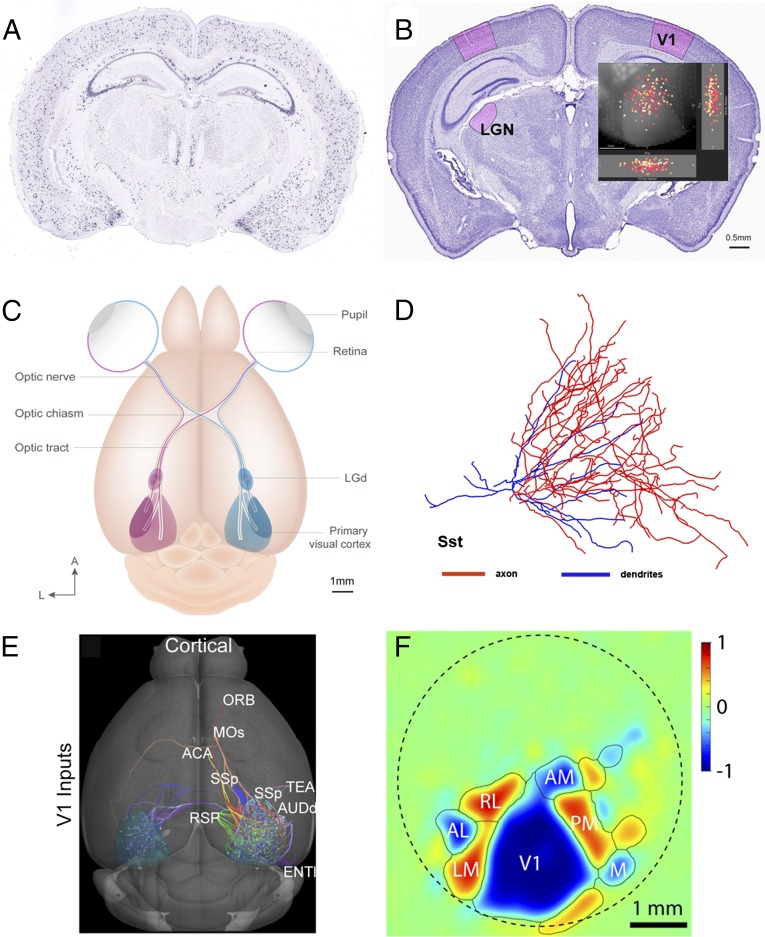
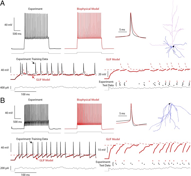
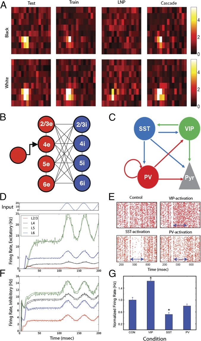
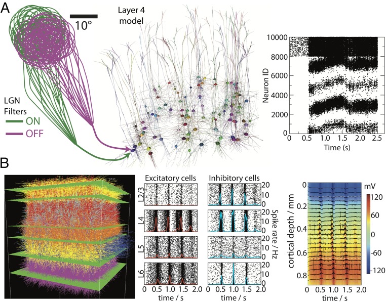
The scientific mission of the Project MindScope is to understand neocortex, the part of the mammalian brain that gives rise to perception, memory, intelligence, and consciousness. We seek to quantitatively evaluate the hypothesis that neocortex is a relatively homogeneous tissue, with smaller functional modules that perform a common computational function replicated across regions. We here focus on the mouse as a mammalian model organism with genetics, physiology, and behavior that can be readily studied and manipulated in the laboratory. We seek to describe the operation of cortical circuitry at the computational level by comprehensively cataloging and characterizing its cellular building blocks along with their dynamics and their cell type-specific connectivities. The project is also building large-scale experimental platforms (i.e., brain observatories) to record the activity of large populations of cortical neurons in behaving mice subject to visual stimuli. A primary goal is to understand the series of operations from visual input in the retina to behavior by observing and modeling the physical transformations of signals in the corticothalamic system. We here focus on the contribution that computer modeling and theory make to this long-term effort.

Keywords: computation; neocortex; neural coding; simulation; visual system.

Fig. 1.

Mapping and analyzing cell type data. (A) A coronal view of the mouse brain showing in situ hybridization data from the Allen Brain Atlas for the Sst gene, a genetic marker for one class of inhibitory interneurons. (B) A view of the brain with the LGN and V1 outlined in red. Inset shows individual V1 Sst cells. (C) Overview of how right (red) and left (blue) visual fields are mapped from the retinas onto the LGN (also referred to as LGd) and from there, onto V1. Ganglion cells target more than 20 other brain structures other than the LGN. (D) A dendritic reconstruction of an Sst V1 interneuron, with its axon in blue and its dendrites in red. (E) V1 receives input from at least 40 distinct anatomical structures (cortical regions are shown) and projects to more than 34 regions (4). (ORB, orbital cortex; MOs, motor cortex; ACA, anterior cerebral artery; SSp, primary somatosensory cortex; TEA, tegmental area; AUDd, dorsal auditory stream; RSP, retrosplenial cortex; and ENT, entorhinal cortex.) (F) Functionally defined visual maps in the mouse visual cortex. V1 is surrounded by other visual regions, such as LM area, AL area, rostrolateral area (RL), anteromedial area (AM), PM area, and medial area (M).

Fig. 2.

Single-cell biophysical and point neuron models. Data from (A) a fluorescently labeled excitatory neuron from genetically modified mouse (Rbp4-Cre tdTomato+) and (B) an SST-labeled inhibitory interneuron (Sst-Cre tdTomato+) (Fig. 1 A and D). A, Upper and B, Upper show examples of $V_m\left(t\right)$ generated by the associated biophysical models. Data (black) and models (red) are shown in response to current injections (gray), with close-up views of individual spikes superimposed. Morphological reconstructions of the modeled cells are shown in A, Right and B, Right, with apical dendrites colored in magenta and other dendrites colored in blue. A, Lower and B, Lower illustrate simpler point models (GLIF) for the same cells, which ignore the detailed morphology structure of the cell. Training data consist of at least three repeats of frozen pink noise: during the fit of the training data (black solid line), the membrane potential (red solid line) and threshold (red dashed line) are computed between spikes. Thus, the spiking histories of the model and the neuron are the same. Test data: during the testing phase, a different instantiation of noise is repeated at least twice, and the resulting spikes (black dots) are compared with the spikes produced by the model (red dots).

Fig. 3.

Population responses in LGN and V1 models. (A) Comparison of the receptive field of a mouse LGN cell using the mean firing rate. At one of 16 × 8 spatial pixels, (A, Upper) a black or (A, Lower) white square was flashed onto an otherwise gray screen. Column 1 shows the spatial receptive field recorded during the test period: a cell with distinct (Upper) off and (Lower) on subfields. Column 2 shows spatial receptive field recorded during the training period from which the models are constructed. The explained variance between test and training sets is $R^2=0.51$. In column 3, the holdout set responses of a single LNP model trained barely reconstruct the visual stimulus ($R^2=0.02$), whereas a cascade model with multiple LNP channels in column 4 has a vastly better performance with $R^2=0.50$. (B) Schematic of a simplified cortical column model [in the work by Potjans and Diesmann (24)]. Mean firing rate dynamics of an LIF simulation of the cortical column (noisy traces) is compared with the coupled population density equation solver DiPDE (smooth traces) for 2 × 4 populations of (D) excitatory and (F) inhibitory neurons (one each in four layers). At 100 ms, one layer 4 subpopulation is driven with an external sinusoidal input (pictured above), simulating LGN input. This simulation results in both linear and nonlinear mean firing rate responses of various populations. The two modeling approaches, DiPDE and LIF simulations, closely agree. (C) Schematic of the cell type-specific connectivity among inhibitory neurons used in the superficial layer of a cortical column model (Pyr, pyramidal neurons). (E) Action potentials of pyramidal neurons in superficial layers in control experiments and under interneuron expressing genes for PV, SST, and VIP cell activation conditions. Arrows indicate the period during which one of three inhibitory populations was activated. (G) The normalized firing rate (and SE) of the pyramidal neurons. *A significant difference between control and the specific simulation conditions (CON, control).

Fig. 4.

Large-scale biophysical simulations of mouse V1. (A) The layer 4 model and simulations. The LGN cells, supplying visual input to layer 4, are modeled as filters that produce spike trains in response to movies in visual space. For each neuron in the layer 4 model, a subset of on and off filters is chosen, and the spike trains generated by these filters are impinging onto the V1 cell; this situation is illustrated for one of the layer 4 neurons. The biophysically detailed model consists of 10,000 neurons; only 1% of these are shown. The simulated neuronal activity in response to visual stimulation with a drifting grating (between 0.5 and 2.5 s) is shown in Right. The first 8,000 neurons are pyramidal cells, and the rest are fast-spiking interneurons. Cells are grouped together according to their orientation preference of the drifting grating. (B, Left) Multilayer network of 24,500 interconnected, biophysically detailed neurons positioned in physical space and color-coded by layer and type. (B, Center) Population rasters and the corresponding spike rates (red lines, excitatory; blue lines, inhibitory neurons) in response to visual stimulus (drifting grating at 2 Hz). (B, Right) The laminar distribution of the simulated extracellular potential (black traces indicate $V_e$ as a function of time and specific depth; color indicates depth $V_e$) in response to neural activity.

Fig. 5.

The Allen Brain Observatory. This in-house project is producing neuronal activity data from genetically identified neuronal populations in the behaving mouse using two-photon calcium imaging. (A) Responses are recorded to a variety of visual stimuli, including gratings, sparse noise, natural images, and natural movies, and across multiple regions, layers, and genetically defined cell types. (B) Example single-neuron response properties. Upper shows receptive fields from locally sparse noise separately for on (white) and off (black) stimuli (Fig. 3A). Lower shows example tuning curves for orientation and spatial frequency obtained from such imaging (in units of DF/F) in response to oriented gratings (cpd, cycles per degree; DF/F, relative change in fluorescence).

References

1. Herculano-Houzel S. The human brain in numbers: A linearly scaled-up primate brain. Front Hum Neurosci. 2009;3(2009):31. - PMC - PubMed
1. Jeon CJ, Strettoi E, Masland RH. The major cell populations of the mouse retina. J Neurosci. 1998;18(21):8936–8946. - PMC - PubMed
1. Tasic B, et al. Adult mouse cortical cell taxonomy revealed by single cell transcriptomics. Nat Neurosci. 2016;19(2):335–346. - PMC - PubMed
1. Oh SW, et al. A mesoscale connectome of the mouse brain. Nature. 2014;508(7495):207–214. - PMC - PubMed
1. Sporns O. Networks of the Brain. MIT Press; Cambridge, MA: 2011.
Publication types
LinkOut - more resources