Causal inference and the data-fusion problem

Abstract

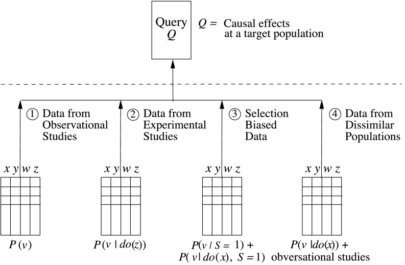
We review concepts, principles, and tools that unify current approaches to causal analysis and attend to new challenges presented by big data. In particular, we address the problem of data fusion-piecing together multiple datasets collected under heterogeneous conditions (i.e., different populations, regimes, and sampling methods) to obtain valid answers to queries of interest. The availability of multiple heterogeneous datasets presents new opportunities to big data analysts, because the knowledge that can be acquired from combined data would not be possible from any individual source alone. However, the biases that emerge in heterogeneous environments require new analytical tools. Some of these biases, including confounding, sampling selection, and cross-population biases, have been addressed in isolation, largely in restricted parametric models. We here present a general, nonparametric framework for handling these biases and, ultimately, a theoretical solution to the problem of data fusion in causal inference tasks.

Keywords: causal inference; counterfactuals; external validity; selection bias; transportability.

Fig. 1.

Prototypical generalization tasks where the goal is, for example, to estimate a causal effect in a target population (Top). Let $V=\left\{X,Y,Z,W\right\}$. There are different designs (Bottom) showing that data come from nonidealized conditions, specifically: (1) from the same population under an observational regime, $P\left(v\right)$; (2) from the same population under an experimental regime when Z is randomized, $P\left(v|do\left(z\right)\right)$; (3) from the same population under sampling selection bias, $P\left(v|S=1\right)$ or $P\left(v|do\left(x\right),S=1\right)$; and (4) from a different population that is submitted to an experimental regime when X is randomized, $P\left(v|do\left(x\right),S=s\right)$, and observational studies in the target population.

Fig. 2.

(A) Graphical model illustrating d-separation and the backdoor criterion. U terms are not shown explicitly. (B) Illustration of the intervention $do\left(X=x\right)$ with arrows toward X cut. (C) Illustration of the spurious paths, which pop out when we cut the outgoing edges from X and need to be blocked if one wants to use adjustment.

Fig. 3.

Graphical models illustrating identification of $Q=P\left(y|do\left(x\right)\right)$ through the use of experiments over an auxiliary variable Z. Identifiability follows from $P\left(x,y|do\left(Z=z\right)\right)$ in A, and it also requires $P\left(v\right)$ in B. Identifiability in models A and B follows from the identifiability of Q in $G_{\overline{Z}}$.

Fig. 4.

Canonical models where selection is treatment dependent in A and B and also outcome dependent in A. More complex models in which $\left\{W_1,W_2\right\}$ and $\left\{Z\right\}$ are sufficient for adjustment, but only the latter is adequate for recovering from selection bias, are shown in C. There is no sufficient set for adjustment without external data in D–F. (D) Example of S-backdoor admissible set. (E and F) Structures with no S-admissible sets that require more involved recoverability strategies involving posttreatment variables.

Fig. 5.

Selection diagrams depicting differences between source and target populations. In A, the two populations differ in age (Z) distributions (so S points to Z). In B, the populations differ in how reading skills (Z) depend on age (an unmeasured variable, represented by the open circle) and the age distributions are the same. In C, the populations differ in how Z depends on X. In D, the unmeasured confounder (bidirected arrow) between Z and Y precludes transportability.

References

1. Pearl J. 2009. Causality: Models, Reasoning, and Inference (Cambridge Univ Press, New York), 2nd Ed.
1. Pearl J. Causal inference in statistics: An overview. Stat Surv. 2009;3:96–146.
1. Pearl J, Glymour M, Jewell NP. 2016 Causal Inference in Statistics: A Primer (Wiley, New York)
1. Angrist J, Imbens G, Rubin D. Identification of causal effects using instrumental variables (with comments) J Am Stat Assoc. 1996;91(434):444–472.
1. Greenland S, Lash T. In: Bias Analysis in Modern Epidemiology. 3rd Ed. Rothman K, Greenland S, Lash T, editors. Lippincott Williams & Wilkins; Philadelphia: 2008. pp. 345–380.