Modeling confounding by half-sibling regression

Abstract

We describe a method for removing the effect of confounders to reconstruct a latent quantity of interest. The method, referred to as "half-sibling regression," is inspired by recent work in causal inference using additive noise models. We provide a theoretical justification, discussing both independent and identically distributed as well as time series data, respectively, and illustrate the potential of the method in a challenging astronomy application.

Keywords: astronomy; causal inference; exoplanet detection; machine learning; systematic error modeling.

Fig. 1.

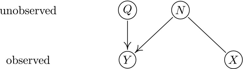
We are interested in reconstructing the quantity Q based on the observables X and Y affected by noise N, using the knowledge that $\left(N,X\right)\mathrm{╨}Q$. Note that the involved quantities need not be scalars, which makes the model more general than it seems at first glance. For instance, we can think of N as a multidimensional vector, some components of which affect only X, some only Y, and some both X and Y.

Fig. 2.

Causal structure from Fig. 1 when relaxing the assumption that X is an effect of N.

Fig. S1.

Example for Prediction based on Noneffects of the Noise Variable. The condition that the regression input X should satisfy $X\mathrm{╨}Q$ rules out its component $X_1$. As a consequence, although $X_3$ is contained in N’s Markov blanket, it is no longer useful as a regression input when predicting Y, because it only contains information about Y conditional on $X_1$. In the end, we are left with only $X_2$ for prediction of Y.

Fig. 3.

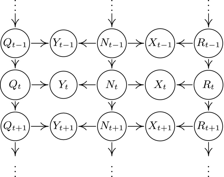
Special case of the time series model. ${\left(Q_t\right)}_t$, ${\left(N_t\right)}_t$, and ${\left(R_t\right)}_t$ are (jointly) independent of each other, but each one may be autocorrelated. Regressing $Y_t$ on ${\left(X_t\right)}_t$ unblocks only paths avoiding $Q_t$: the estimate ${\widehat{Y}}_t≔Y_t-E\left[Y_t|{\left(X_t\right)}_t\right]$ of $Y_t$ does not regress out any variability caused by $Q_t$ and is more accurate than the i.i.d. estimate $Y_t-E\left[Y_t|X_t\right]$. Regressing $Y_t$ on $Y_{t-1}$ unblocks two paths: one avoiding $Q_t$, and the other not. The first may enhance the estimate of $Q_t$; the second, however, may worsen it. In general, the contribution of both parts cannot be separated. However, they can for particular time series ${\left(Q_t\right)}_t$.

Fig. 4.

Simulated transit reconstruction using half-sibling regression for time series, but without regressing on $X_t$. From bottom to top: ${\left(F_t\right)}_t$, ${\left(Y_t\right)}_t$, ${\left({\widehat{Y}}_t\right)}_t$ with $Y_t=S_t{F}_t$, and ${\widehat{Q}}_t≔{\left(Y_t-{\widehat{Y}}_t\right)}_t$. The estimate ${\widehat{Y}}_t$ was trained using ridge regression with regularization parameter $\mathit{\lambda }=0.1$. Transits were also present in the training set. Note that the transit itself is preserved. However, some artifacts (here: bumps) are introduced to the right and left of the transit.

Fig. 5.

(Left) We observe a variable $X=g\left(N\right)+R$ with invertible function g. If the variance of R decreases, the reconstruction of Q improves because it becomes easier to remove the influence $f\left(N\right)$ of the noise N from the variable $Y=f\left(N\right)+Q$ by using X; see Proposition 4. (Right) A similar behavior occurs with increasing the number d of predictor variables $X_i=g_i\left(N\right)+R_i$; see Proposition 5. Both plots show 20 scenarios, each connected by a thin line.

Fig. 6.

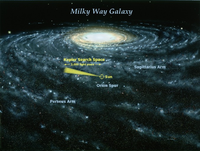
View of the Milky Way with position of the Sun and depiction of the Kepler search field. Image courtesy of © Jon Lomberg.

Fig. S2.

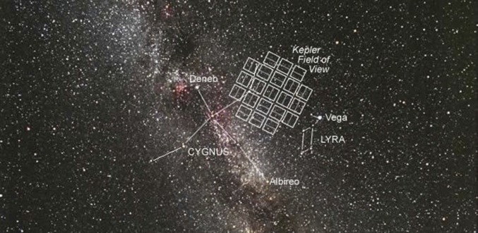
Kepler search field as seen from Earth, located close to the Milky Way plane, in a star-rich area near the constellation Cygnus. Image courtesy of NASA/Carter Roberts/Eastbay Astronomical Society.

Fig. S3.

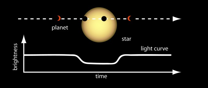
Sketch of the transit method for exoplanet detection. As a planet passes in front of its host star, we can observe a small dip in the apparent star brightness. Image courtesy of NASA Ames.

Fig. S4.

Stars on the same CCD share systematic errors. A and B show pixel fluxes (brightnesses) for two stars: KIC 5088536 (A) and KIC 5949551 (B); here, KIC stands for Kepler Input Catalog. Both stars lie on the same CCD but are far enough apart so that there is no stray light from one affecting the other. Each panel shows the pixels contributing to the respective star. Note that there exist similar trends in some pixels of these two stars, caused by systematic errors.

Fig. 7.

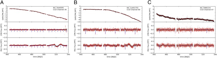
Corrected fluxes using our method, for three example stars, spanning the main magnitude (brightness) range encountered. We consider a bright star (A), a star of moderate brightness (B), and a relatively faint star (C). SAP stands for Simple Aperture Photometry (in our case, a relative flux measure computed from summing over the pixels belonging to a star). In A−C, Top shows the SAP flux (black) and the cpm regression (red), i.e., our prediction of the star from other stars. Middle shows the cpm flux corrected using the regression (for details, see Applications, Exoplanet Light Curves), and Bottom shows the PDC flux (i.e., the default method). The cpm flux curve preserves the exoplanet transits (little downward spikes), while removing a substantial part of the variability present in the PDC flux. All x axes show time, measured in days since January 1, 2009.

Fig. 8.

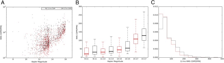
Comparison of the proposed method (cpm) to the Kepler PDC method in terms of CDPP (see Applications, Exoplanet Light Curves). A shows our performance (red) vs. the PDC performance in a scatter plot, as a function of star magnitude (note that larger magnitude means fainter stars, and smaller values of CDPP indicate a higher quality as measured by CDPP). B bins the same dataset and shows box plots within each bin, indicating median, top quartile, and bottom quartile. The red box corresponds to cpm, and the black box refers to PDC. C shows a histogram of CDPP values. Note that the red histogram has more mass toward the left (i.e., smaller values of CDPP), indicating that our method overall outperforms PDC, the Kepler “gold standard.”

References

-
- Schölkopf B, et al. On causal and anticausal learning. In: Langford J, Pineau J, editors. Proceedings of the 29th International Conference on Machine Learning (ICML) Omnipress; New York: 2012. pp. 1255–1262.
- Pearl J. Causality. Cambridge Univ Press; New York: 2000.
- Spirtes P, Glymour C, Scheines R. Causation, Prediction, and Search. 2nd Ed MIT Press; Cambridge, MA: 1993.
- Aldrich J. Autonomy. Oxf Econ Pap. 1989;41(1):15–34.
- Hoover KD. Causality in economics and econometrics. In: Durlauf SN, Blume LE, editors. Economics and Philosophy. 2nd Ed. Vol 6 Palgrave Macmillan; New York: 2008.
Publication types
LinkOut - more resources
Full Text Sources
Other Literature Sources