

doi: 10.1371/journal.pone.0158239.
eCollection 2016.
Toward a More Efficient Implementation of Antifibrillation Pacing
Affiliations
- PMID: 27391010
- PMCID: PMC4938213
- DOI: 10.1371/journal.pone.0158239
Item in Clipboard
Toward a More Efficient Implementation of Antifibrillation Pacing
PLoS One.
.
Abstract
We devise a methodology to determine an optimal pattern of inputs to synchronize firing patterns of cardiac cells which only requires the ability to measure action potential durations in individual cells. In numerical bidomain simulations, the resulting synchronizing inputs are shown to terminate spiral waves with a higher probability than comparable inputs that do not synchronize the cells as strongly. These results suggest that designing stimuli which promote synchronization in cardiac tissue could improve the success rate of defibrillation, and point towards novel strategies for optimizing antifibrillation pacing.
Conflict of interest statement
Figures
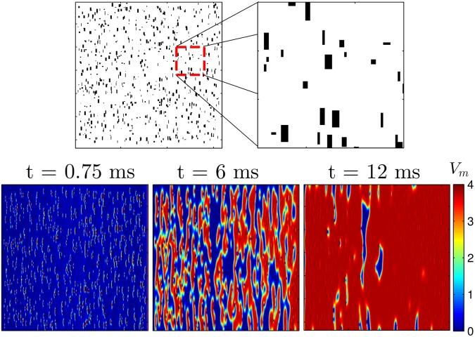
In the bottom panels a voltage gradient of 1500 units applied from left to right to a 2D sheet of quiescent cells Eq (2) for a duration of 1.5 ms. Because of the removal of the gap junctions, virtual electrodes start to form soon after the voltage gradient is applied. By 12 ms, nearly all cells in the domain have been excited. The colorbar presented here applies to all simulations using the Karma model.
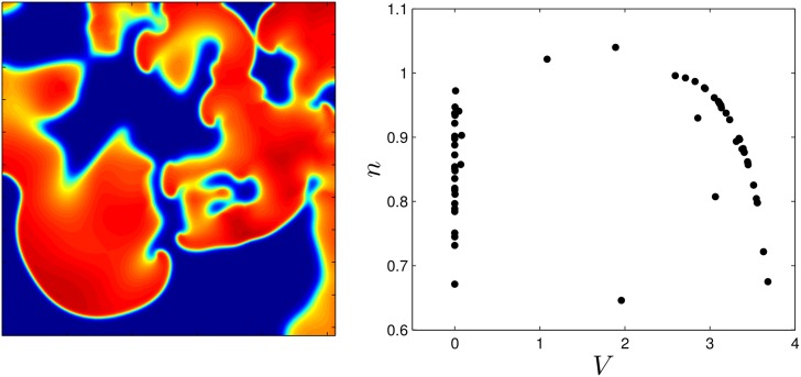
The right panel shows the states of 250 cells, chosen to provide a uniform sampling over the grid.
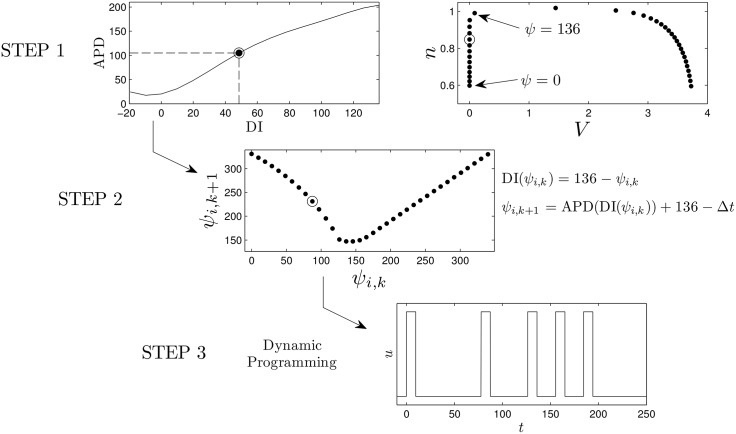
First, the transient attractor is discretized into points that are equally spaced in time. In the top panel, the cell repolarizes at ψ = 136 which corresponds to a DI of zero (i.e. the state at which cell has just repolarized). A mapping based on giving an excitatory stimulus, ψi,k → ψi,k+1, can be calculated using the equations in step 2. From the numerically determined map using the Karma model, we find that if a cell has been recently reexcited, another stimulus does not affect the time at which the cell repolarizes (i.e. ψi,k+1 = ψi,k − Δt). In steps 1 and 2, we highlight the information required to calculate the excitation map with circled datapoints. Finally, using the excitation map, the dynamic programming procedure outlined here can be be used to calculate an optimal pulsing pattern. Note that multiple maps for different stimuli can be calculated and included in the optimization procedure.
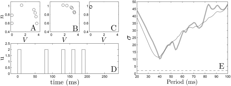
Panels (A)-(C) show the optimal states of the 7 cell system at times 0, 100, and 220 ms, respectively. Panel (D) shows the optimal pulse train obtained from dynamic programming. In panel (E), we apply five pulses at constant period to the same system of 7 cells (grey line) and a system with one cell at each of the 36 states (black line) along the transient attractor as initial conditions. We see qualitative agreement between both plots. The dashed line represents the standard deviation obtained from optimal pulse train on the 7 cell system.
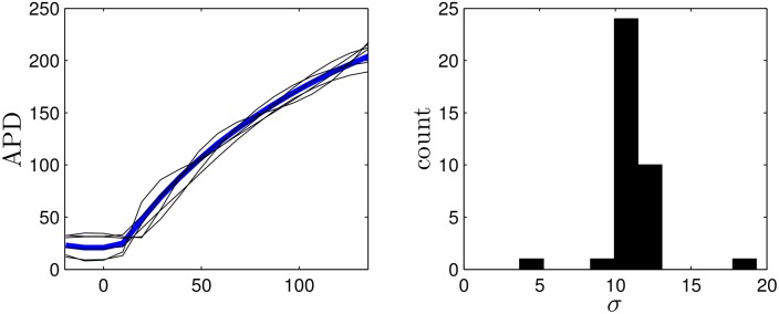
The optimization process is performed on other randomly generated curves to gauge the robustness of the optimization algorithm. Five representative curves are shown as black lines. The right panel shows the synchronization from resulting optimal stimuli applied to 36 uncoupled cells reported as the standard deviation of their repolarization times.
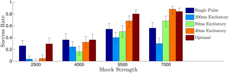
Error bars represent a confidence interval corresponding to one standard deviation. Overall, the synchronization predicted from panel E of Fig 4 is correlated to the success rate for each shock strategy. For all multiple pulse trials, the shock strength is reported as the difference between the maximum and minimum extracellular voltages. For the single defibrillating pulse, the induced voltage gradient is to keep energy consumption equivalent to that of the other trials, assuming energy consumption is proportional to ∫ (Shock Strength)2
dt.
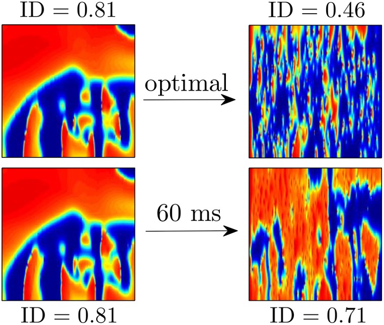
In the top panels, using the optimal stimulus yields an ID of 0.46 40 ms after the final pulse is applied. The distribution of excited and quiescent cells is similar throughout the tissue, making it less likely that the remaining wave fronts will find a reentrant pathway. In the bottom panel, using the 60 ms pulsed stimulus yields an ID of 0.62 40 ms after the final pulse is applied. The large connected regions of excited and quiescent tissue make it more likely that the remaining wave fronts will produce new reentrant waves.
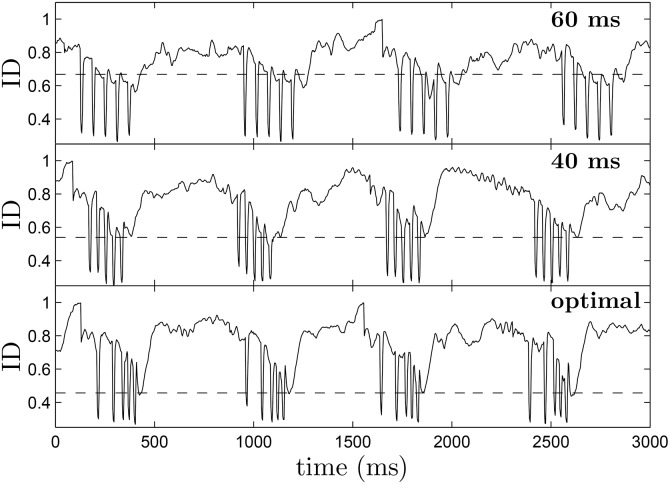
During each pulse, the ID drops suddenly, because of the pattern of hyperpolarization and depolarization that the virtual electrodes create. If the ID soon after the final pulse is small, it indicates that excited and quiescent tissue are thoroughly mixed, making it less likely for spirals to reenter. Over multiple trials, the average value of ID 30 ms after the final pulse is 0.456, 0.539, and 0.668 for the optimal, 40 ms pulsed, and 60 ms pulsed strategies, respectively, as indicated by dotted lines in each figure. These results are consistent with the synchronization that would be expected from panel (E) of Fig 4.
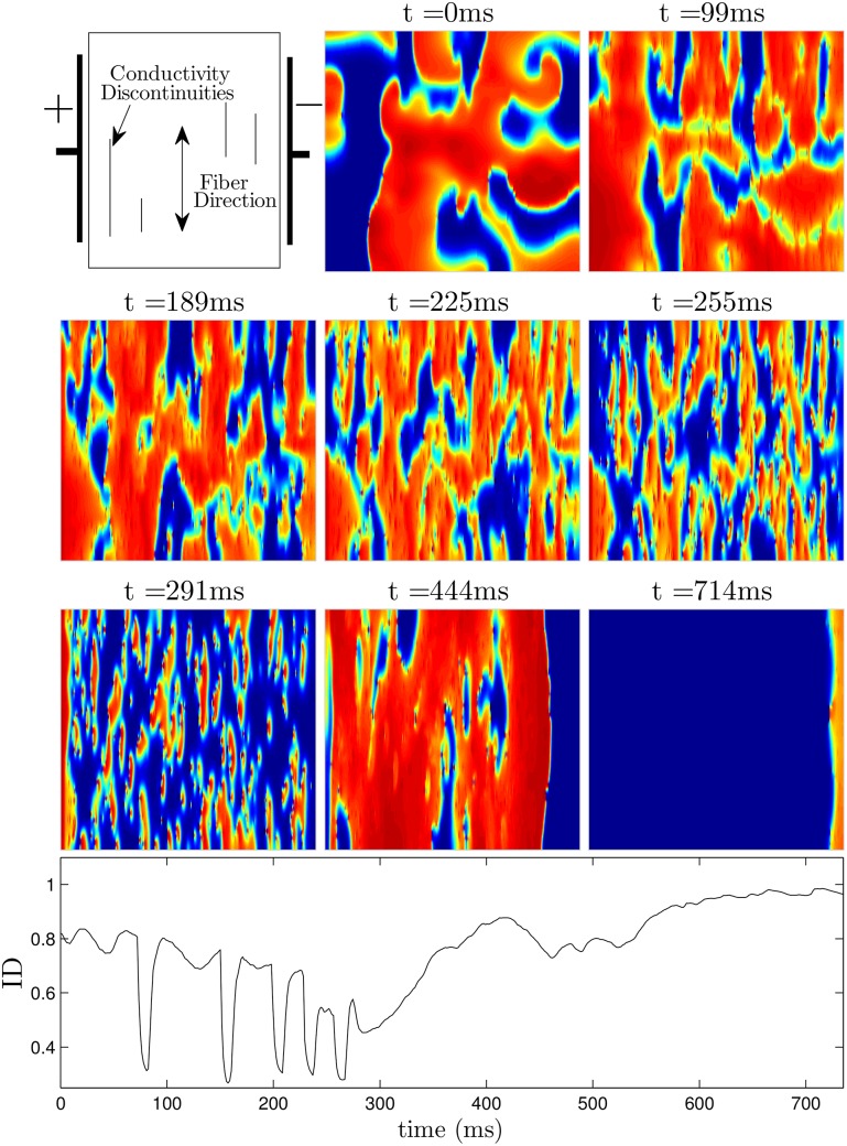
The panel at t = 0ms shows the system before a defibrillating stimulus is applied. The next five panels show the system approximately 30ms after successive pulses are applied. Notice that soon after the last pulse is applied at t = 291ms, the ID is close to 0.45, indicating that the excited and quiescent cells are spread evenly throughout the medium. In the final two panels, any remaining spiral waves are extinguished. The bottom panel shows ID as a function of time. See also S2 File.
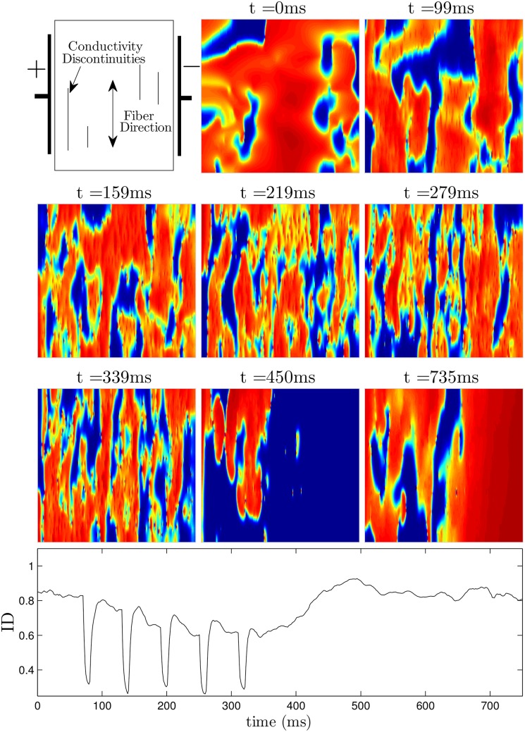
The panel at t = 0ms shows the system before a defibrillating stimulus is applied. The next five panels show the system approximately 30ms after successive pulses are applied. Notice that soon after the last pulse is applied at t = 339ms, the ID is around 0.65, indicating that there will likely be pathways for spiral waves to reenter, as shown in the final two panels. See also S3 File.
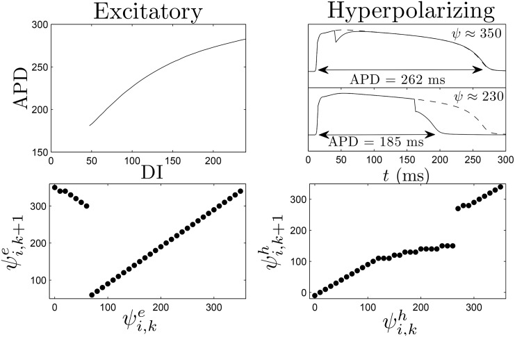
The top-right shows that a strictly hyperpolarizing stimulus applied soon after a cell is excited (ψ ≈ 350) has little effect on the time at which the cell repolarizes, while the same stimulus applied later (ψ ≈ 230) will hasten repolarization. The dashed line shows the transmembrane voltage if the strictly hyperpolarizing stimulus had not been applied. The bottom-right panel shows the hyperpolarization map, which is calculated for each discretized phase.
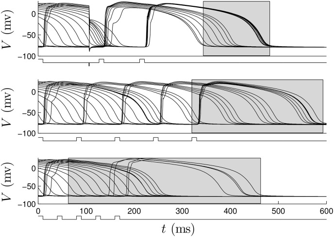
The grey boxes represent the distribution of times at which cells repolarize. In the signals below the voltage traces, positive pulses represent excitatory perturbations. The negative pulse in the top panel occurs at approximately 100 ms and represents a strictly hyperpolarizing perturbation.
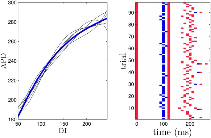
The optimization is performed using randomly modified APD restitution curves and hyperpolarization maps as described in the text. Five representative APD curves are shown in black. The right panel gives the resulting optimal pulsing pattern calculated over 98 trials. Red marks indicate excitatory pulses and blue marks represent hyperpolarizing pulses. For comparison, the optimal pulse series using the true data has excitatory pulses at 0, 120, and 200 ms and a hyperpolarizing pulse at 100 ms.
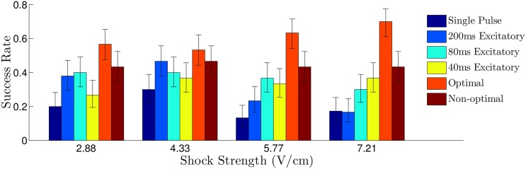
Error bars represent a confidence interval corresponding to one standard deviation. For all multiple pulse trials, the shock strength is reported as the voltage gradient induced during an excitatory pulse. For the single defibrillating pulse, the induced voltage gradient is to keep energy consumption equivalent to that of the strictly excitatory trials, assuming energy consumption is proportional to ∫ (Shock Strength)2
dt.
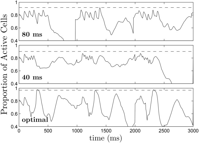
Dashed lines at 0.968, 0.903, and 0.918 for the optimal, 40 ms pulsed, and 80 ms pulsed strategies, respectively represent the maximum proportion of active cells, averaged over multiple trials.
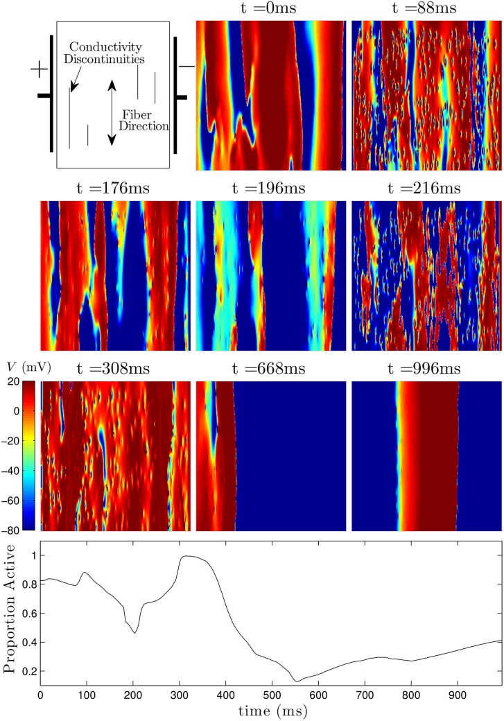
The pulsing strategy manipulates the tissue so that soon after the final pulse at t = 308ms, most of the cells are excited, and spiral waves cannot continue to propagate through the medium. The bottom panel shows the proportion of active cells as a function of time. The colorbar presented here applies to all simulations using the ten Tusscher-Panfilov model.
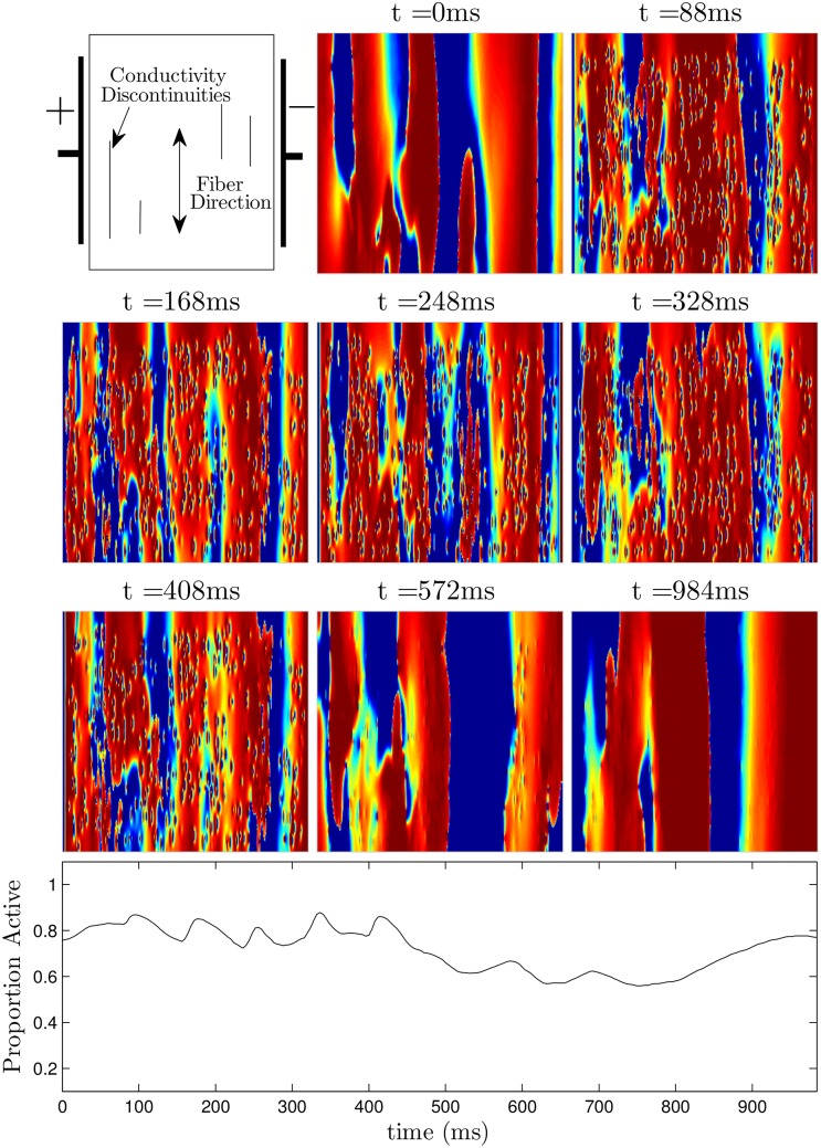
Soon after the final pulse at t = 408ms, large portions of tissue are still quiescent, allowing spiral waves to persist. The bottom panel shows the proportion of active cells as a function of time.
Similar articles
-
Turbulence control with local pacing and its implication in cardiac defibrillation.Chaos. 2007 Mar;17(1):015107. doi: 10.1063/1.2713688. Chaos. 2007. PMID: 17411264 Review.
-
Low energy defibrillation in human cardiac tissue: a simulation study.Biophys J. 2009 Feb 18;96(4):1364-73. doi: 10.1016/j.bpj.2008.11.031. Biophys J. 2009. PMID: 19217854 Free PMC article.
-
European Resuscitation Council Guidelines for Resuscitation 2010 Section 3. Electrical therapies: automated external defibrillators, defibrillation, cardioversion and pacing.Resuscitation. 2010 Oct;81(10):1293-304. doi: 10.1016/j.resuscitation.2010.08.008. Resuscitation. 2010. PMID: 20956050 No abstract available.
-
Alternans and the influence of ionic channel modifications: Cardiac three-dimensional simulations and one-dimensional numerical bifurcation analysis.Chaos. 2007 Mar;17(1):015104. doi: 10.1063/1.2715668. Chaos. 2007. PMID: 17411261
-
Defibrillation of the heart: insights into mechanisms from modelling studies.Exp Physiol. 2006 Mar;91(2):323-37. doi: 10.1113/expphysiol.2005.030973. Epub 2006 Feb 9. Exp Physiol. 2006. PMID: 16469820 Review.
Cited by
-
Terminating spiral waves with a single designed stimulus: Teleportation as the mechanism for defibrillation.Proc Natl Acad Sci U S A. 2022 Jun 14;119(24):e2117568119. doi: 10.1073/pnas.2117568119. Epub 2022 Jun 9. Proc Natl Acad Sci U S A. 2022. PMID: 35679346 Free PMC article.
References
-
- Jacq F, Foulldrin G, Savouré A, Anselme F, Baguelin-Pinaud A, Cribier A, et al. A comparison of anxiety, depression and quality of life between device shock and nonshock groups in implantable cardioverter defibrillator recipients. General Hospital Psychiatry. 2009;31(3):266–273. 10.1016/j.genhosppsych.2009.01.003 - DOI - PubMed
-
- Suzuki T, Shiga T, Kuwahara K, Kobayashi S, Suzuki S, Nishimura K, et al. Prevalence and Persistence of Depression in Patients with Implantable Cardioverter Defibrillator: A 2-year Longitudinal Study. Pacing and Clinical Electrophysiology. 2010;33(12):1455–1461. 10.1111/j.1540-8159.2010.02887.x - DOI - PubMed
MeSH terms
LinkOut - more resources
Full Text Sources
Other Literature Sources
Medical
